Querying the CosmoDC2 Mock v1 Catalogs

This tutorial demonstrates how to access and query the CosmoDC2 Mock v1 catalogs using IRSA’s Table Access Protocol (TAP) service. Background information on the catalogs is available on the IRSA CosmoDC2 page.

The catalogs are served through IRSA’s Virtual Observatory–standard TAP interface, which you can access programmatically in Python via the PyVO library. TAP queries are written in the Astronomical Data Query Language (ADQL) — a SQL-like language designed for astronomical catalogs (see the ADQL specification).

If you are new to PyVO’s query modes, the documentation provides a helpful comparison between synchronous and asynchronous execution: PyVO: Synchronous vs. Asynchronous Queries

Tips for Working with CosmoDC2 via TAP¶

• Use indexed columns for fast queries. CosmoDC2 is indexed on the following fields: ra, dec, redshift, mag*_lsst, halo_mass, stellar_mass Queries involving these columns generally return much faster.

• Ensure your positional queries fall within the survey footprint. CosmoDC2 covers the area specified by the following (R.A., decl.) coordinate pairs (J2000): (71.46,−27.25), (52.25,−27.25), (73.79,−44.33), (49.42,−44.33).

• Avoid overloading the TAP service. Preferentially use asynchronous queries for long running queries to avoid timing out. The whole system will slow down if a lot of people are using it for large queries, or if you decide to kick off many large queries at the same time.

# Uncomment the next line to install dependencies if needed.
# !pip install numpy matplotlib pyvo

import pyvo as vo
import numpy as np
import matplotlib.mlab as mlab
import matplotlib.pyplot as plt

service = vo.dal.TAPService("https://irsa.ipac.caltech.edu/TAP")

1. List the available DC2 tables¶

tables = service.tables
for tablename in tables.keys():
    if not "tap_schema" in tablename:
        if "dc2" in tablename:
            tables[tablename].describe()

cosmodc2mockv1
    CosmoDC2MockV1 Catalog - unabridged, spatially partitioned

cosmodc2mockv1_heavy
    CosmoDC2MockV1 Catalog - stellar mass > 10^7 Msun

cosmodc2mockv1_new
    CosmoDC2MockV1 Catalog - unabridged

2. Choose the DC2 catalog you want to work with.¶

IRSA currently offers 3 versions of the DC2 catalog.

• cosmodc2mockv1_new has been optimized to make searches with constraints on stellar mass and redshift fast.

• cosmodc2mockv1 has been optimized to make searches with spatial constraints fast.

• cosmodc2mockv1_heavy is the same as cosmodc2mockv1_new, except that it does not contain galaxies with stellar masses <= 10^7 solar masses.

If you are new to the DC2 catalog, we recommend that you start with cosmodc2mockv1_heavy

# Choose the abridged table to start with.
# Queries should be faster on smaller tables.

tablename = 'cosmodc2mockv1_heavy'

3. What is the default maximum number of rows returned by the service?¶

This service will return a maximum of 2 billion rows by default.

service.maxrec

This default maximum can be changed, and there is no hard upper limit to what it can be changed to.

print(service.hardlimit)

None

4. List the columns in the chosen table¶

This table contains 301 columns.

columns = tables[tablename].columns
print(len(columns))

301

Let’s learn a bit more about them.

for col in columns:
    print(f'{f"{col.name}":30s}  {col.description}')

5. Retrieve a list of galaxies within a small area¶

Since we know that cosmoDC2 is a large catalog, we can start with a spatial search over a small square area. The ADQL that is needed for the spatial constraint is shown below. We then show how to make a redshift histogram of the sample generated.

# Setup the query
adql = f"""
SELECT redshift
FROM {tablename}
WHERE CONTAINS(
    POINT('ICRS', ra, dec),
    CIRCLE('ICRS', 54.0, -37.0, 0.05)
) = 1
"""

cone_results = service.run_sync(adql)

#how many redshifts does this return?
print(len(cone_results))

10640

# Now that we have a list of galaxy redshifts in that region, we can
# create a histogram of the redshifts to see what redshifts this survey includes.

# Plot a histogram
num_bins = 20
# the histogram of the data
n, bins, patches = plt.hist(cone_results['redshift'], num_bins,
                            facecolor='blue', alpha = 0.5)
plt.xlabel('Redshift')
plt.ylabel('Number')
plt.title(f'Redshift Histogram {tablename}')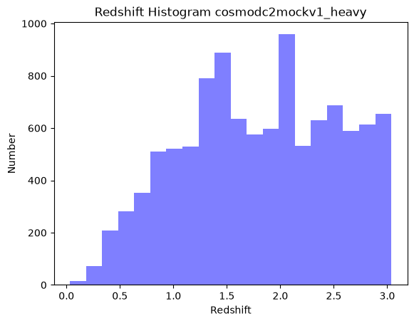

We can see form this plot that the simulated galaxies go out to z = 3.

6. Visualize galaxy colors: redshift search¶

First, we’ll do a narrow redshift cut with no spatial constraint. Then, from that redshift sample we will visualize the galaxy main sequence at z = 2.0.

# Setup the query
adql = f"""
SELECT TOP 50000
    mag_r_lsst,
    (mag_g_lsst - mag_r_lsst) AS color,
    redshift
FROM {tablename}
WHERE redshift BETWEEN 1.95 AND 2.05
"""
redshift_results = service.run_sync(adql)

redshift_results

# Construct a 2D histogram of the galaxy colors
plt.hist2d(redshift_results['mag_r_lsst'], redshift_results['color'],
            bins=100, cmap='plasma', cmax=500)

# Plot a colorbar with label.
cb = plt.colorbar()
cb.set_label('Number')

# Add title and labels to plot.
plt.xlabel('LSST Mag r')
plt.ylabel('LSST rest-frame g-r color')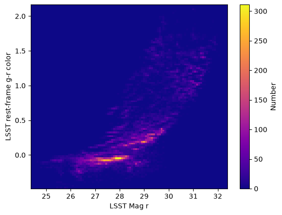

7. Suggestions for further queries:¶

TAP queries are extremely powerful and provide flexible ways to explore large catalogs like CosmoDC2, including spatial searches, photometric selections, cross-matching, and more. However, many valid ADQL queries can take minutes or longer to complete due to the size of the catalog, so we avoid running those directly in this tutorial. Instead, the examples here have so far focused on fast, lightweight queries that illustrate the key concepts without long wait times. If you are interested in exploring further, here are some additional query ideas that are scientifically useful but may take longer to run depending on server conditions.

Count the total number of redshifts in the chosen table¶

The answer for the 'cosmodc2mockv1_heavy' table is 597,488,849 redshifts.

adql = f"SELECT count(redshift) FROM {tablename}"

Count galaxies in a sky region (cone search)¶

Generally useful for: estimating source density, validating spatial footprint, testing spatial completeness.

adql = f"""
SELECT COUNT(*)
FROM {tablename}
WHERE CONTAINS(POINT('ICRS', ra, dec), CIRCLE('ICRS', 54.2, -37.5, 0.2)) = 1
"""

Retrieve only a subset of columns (recommended for speed) and rows¶

This use of “TOP 5000” just limits the number of rows returned. Remove it if you want all rows, but keep in mind such a query can take a much longer time.

adql = f"""
SELECT TOP 5000
    ra,
    dec,
    redshift,
    stellar_mass
FROM {tablename}"""

Explore the stellar–halo mass relation¶

adql = f"""
SELECT TOP 500000
    stellar_mass,
    halo_mass
FROM {tablename}
WHERE halo_mass > 1e11"""

Find the brightest galaxies at high redshift¶

Return the results in ascending (ASC) order by r band magnitude.

adql = f"""
SELECT TOP 10000
    ra, dec, redshift, mag_r_lsst
FROM {tablename}
WHERE redshift > 2.5
ORDER BY mag_r_lsst ASC
"""

About this notebook¶

Author: IRSA Data Science Team, including Vandana Desai, Jessica Krick, Troy Raen, Brigitta Sipőcz, Andreas Faisst, Jaladh Singhal

Updated: 2025-12-16

Contact: the IRSA Helpdesk with questions or reporting problems.

Runtime: As of the date above, this notebook takes about 2 minutes to run to completion on a machine with 8GB RAM and 2 CPU. Large variations in this runtime can be expected if the TAP server is busy with many queries at once.