Learning Goals
By the end of this tutorial, you will be able to:
Access the Euclid Q1 cluster catalog and MER multi-band image data from IRSA.
Apply DBSCAN to identify galaxy overdensities and confirm cluster membership.
Analyze color-magnitude diagrams to characterize cluster and field galaxy populations.
Cross-match Euclid photometric data with NED to independently validate cluster detections.
Introduction
Galaxy clusters are the most massive gravitationally bound structures in the universe, and studying them reveals how large-scale structure forms and how environment shapes galaxy evolution. Euclid is exceptionally well-suited for this science. Its wide-field imager covers large areas of sky in a single pointing, making it efficient at finding rare, massive clusters across a range of redshifts. The combination of a deep optical VIS band — reaching sub-arcsecond resolution — with simultaneous near-infrared Y, J, and H photometry means that cluster member galaxies can be cleanly separated from foreground and background objects using photometric redshifts, even at z ~ 0.5 and beyond where cluster members are faint and red. The red sequence of passively evolving ellipticals that dominates cluster cores stands out sharply in Euclid color space, and the infrared bands trace stellar mass rather than recent star formation, giving a more complete census of cluster membership. Together these properties make Euclid data ideal for detecting clusters, characterising their galaxy populations, and comparing cluster members to field galaxies.
This tutorial explores galaxy clusters in the Euclid Q1 merged multi-wavelength mosaic (MER) image data to demonstrate cluster detection and validation techniques.
We select a cluster from this paper (https://
Input
Euclid Q1 cluster catalog (PZWav and AMICO detections from arXiv:2503.19196)
Euclid Q1 MER multi-band mosaic images
Euclid Q1 photometric galaxy catalogs
Output
Confirmed galaxy cluster and control field detection using DBSCAN
Color-magnitude diagrams comparing cluster and field populations
Cross-matched redshift comparison between Euclid and NED
Imports
# Uncomment the next line to install dependencies if needed.
# !pip install pandas[xml] numpy matplotlib s3fs tqdm astropy astroquery pyvo requests scikit-learn
import os
import time
import pandas as pd
import numpy as np
import matplotlib.pyplot as plt
import requests
import json
import s3fs
from tqdm import tqdm
from concurrent.futures import ThreadPoolExecutor
# Astropy imports
from astropy import units as u
from astropy.coordinates import SkyCoord, match_coordinates_sky, search_around_sky
from astropy.io import fits
from astropy.nddata import Cutout2D
from astropy.wcs import WCS
from astropy.visualization import ImageNormalize, PercentileInterval, AsinhStretch
from astropy.utils.data import download_file
from astropy.table import QTable
# External data access
from astroquery.ipac.irsa import Irsa
from astroquery.ipac.ned import Ned
from astroquery.exceptions import RemoteServiceError
from pyvo.dal import DALQueryError
from requests.exceptions import Timeout, ConnectionError
# Machine learning
from sklearn.cluster import DBSCAN
# Statistics and signal processing
from scipy.stats import gaussian_kde
from scipy.ndimage import gaussian_filter1d, median_filter
Number = u.def_unit("Number")
u.add_enabled_units([Number])<astropy.units.core._UnitContext at 0x7fb9d36bef30>1. Loading the Cluster Catalog
The Euclid Q1 cluster catalog from arXiv:2503.19196 is not available as a direct download, so we read it from the HTML-rendered version of the paper. The HTML table sometimes contains Unicode formatting artifacts in the coordinate columns (e.g., typographic minus signs in negative declinations), which we normalize before use. The catalog contains 35 galaxy clusters with photometric redshifts, coordinates, and richness estimates from the PZWav and AMICO algorithms.
# Load the Euclid Q1 cluster catalog (https://arxiv.org/abs/2503.19196)
url = "https://ar5iv.labs.arxiv.org/html/2503.19196"
fname = "euclid_q1_clusters.csv"
download_path = "data"
os.makedirs(download_path, exist_ok=True)

csv_path = os.path.join(download_path, fname)
if os.path.exists(csv_path):
    df = pd.read_csv(csv_path)
else:
    # Read all tables from the arXiv HTML rendering
    dfs = pd.read_html(url)

    # Select the table containing the cluster catalog
    df = dfs[1].copy()

    # Drop the spurious row that contains units instead of data
    df = df[df["ID"].notna()]

    # Normalize Unicode minus signs and extract numeric RA/Dec values
    # (HTML tables sometimes concatenate values or include formatting artifacts)
    for col in ["RAPZWav", "DecPZWav"]:
        df[col] = (
            df[col].astype(str)
                   .str.replace("−", "-", regex=False)
                   .str.extract(r"([-+]?\d+(?:\.\d+)?)")[0]
                   .astype(float)
        )

    # Rename LaTeX-style column names to clean, code-friendly names
    df = df.rename(columns={
        "zPZWavz_{\\mathrm{PZWav}}": "zPZWav",
        "zAMICOz_{\\mathrm{AMICO}}": "zAMICO",
        "λPmem\\lambda_{\\mathrm{Pmem}}": "lambdaPmem",
    })

    df.to_csv(csv_path, index=False)

print(f"Dataset shape: {df.shape}")
df.head(3)
Dataset shape: (35, 13)
2. A Cluster and Control Field Selection
We use cluster EUCL-Q1-CL-1, a richly populated galaxy overdensity at z = 0.55 detected in the Euclid Q1 data. We also need a control field — a region of sky with no known clusters — to characterise the field galaxy population for comparison.
# Select cluster EUCL-Q1-CL-1 from the catalog
cluster = df[df['ID'] == 'EUCL-Q1-CL-1'].iloc[0]
cluster_ra  = cluster['RAPZWav']
cluster_dec = cluster['DecPZWav']
cluster_z   = cluster['zPZWav']
cluster_coord = SkyCoord(ra=cluster_ra, dec=cluster_dec, unit='deg')

print(f"Cluster: {cluster['NAME']}")
print(f"  RA: {cluster_ra:.4f}°, Dec: {cluster_dec:.4f}°, z = {cluster_z:.2f}")

# Query the MER image catalog for this position
cluster_mer_images = Irsa.query_sia(pos=(cluster_coord, 2.0 * u.arcmin), collection='euclid_DpdMerBksMosaic')
cluster_mer_images = cluster_mer_images[
    (cluster_mer_images['facility_name'] == 'Euclid') &  #also contains data from other telescopes, so be specific
    (cluster_mer_images['dataproduct_subtype'] == 'science')
]
print(f"  Found {len(cluster_mer_images)} MER science images")
Cluster: EUCL-Q1-CL J041724.90−-474849.7
RA: 64.3521°, Dec: -47.8150°, z = 0.55
Found 4 MER science images
A control field is a sky region with no known galaxy clusters, used to characterise the general field galaxy population for comparison with the cluster environment.
We select the control field by picking a random offset direction from a catalog cluster and rejecting any candidate control field that falls within min_distance_arcmin of any known cluster.
The MER mosaic is organised into tiles, and positions near tile boundaries may overlap two tiles, which complicates downloading. We also check that both the cluster and control field each fall on exactly one tile before proceeding.
We fix the random seed so the tutorial gives reproducible results by always picking the same control field. To explore a different control field, change the seed value or remove the seed entirely.
def check_mer_tile_requirement(coord, search_radius=2.0):
    """Check whether a sky coordinate is covered by exactly 4 Euclid MER science images.

    The Euclid MER mosaic is organized into tiles. A position inside a single
    tile returns exactly 4 images, one per photometric band (VIS, Y, J, H).
    Positions near tile boundaries may overlap two tiles and return more than 4
    images; those are rejected to avoid partial-coverage complications.

    Parameters
    ----------
    coord : `~astropy.coordinates.SkyCoord`
        Sky coordinate to check.
    search_radius : float, optional
        Radius in arcminutes within which to search for MER images. Default is 2.0.

    Returns
    -------
    valid : bool
        True if exactly 4 science images are found; False otherwise.
    mer_images : `~astropy.table.Table` or None
        Table of matching MER image records, or None if the query failed.
    """
    try:
        mer_images = Irsa.query_sia(pos=(coord, search_radius * u.arcmin), collection='euclid_DpdMerBksMosaic')
        mer_images = mer_images[(mer_images['facility_name'] == 'Euclid') & (mer_images['dataproduct_subtype'] == 'science')]

        if len(mer_images) == 4:
            print(f"  ✓ Found exactly 4 images for coordinates")
            return True, mer_images
        else:
            print(f"  ✗ Found {len(mer_images)} images (expected 4) - trying next location")
            return False, mer_images
    except (DALQueryError, Timeout, ConnectionError, OSError) as e:
        print(f"  ✗ Error querying MER tiles: {e}")
        return False, None
def find_control_field(cluster_df, cluster_ra, cluster_dec, min_distance_arcmin=15, max_attempts=100):
"""Find a random control field offset from the known cluster catalog.
Generates candidate control fields by randomly offsetting 25–35 arcmin from
a randomly chosen catalog cluster in a random direction. Each candidate is
accepted only if it lies at least ``min_distance_arcmin`` away from every
cluster in the catalog, ensuring the control field is a genuine blank field
representative of the general galaxy population.
RA offsets are corrected for the cosine of the declination so that angular
separations are accurate. If no valid field is found within ``max_attempts``,
a fallback position directly offset from the target cluster is returned.
Parameters
----------
cluster_df : `pandas.DataFrame`
Cluster catalog with columns ``RAPZWav`` and ``DecPZWav`` (degrees).
cluster_ra : float
RA of the target cluster in degrees (used for the fallback only).
cluster_dec : float
Dec of the target cluster in degrees (used for the fallback only).
min_distance_arcmin : float, optional
Minimum angular separation in arcminutes from all catalog clusters.
Default is 15.
max_attempts : int, optional
Maximum number of random candidates to try before falling back.
Default is 100.
Returns
-------
control_ra : float
RA of the selected control field in degrees.
control_dec : float
Dec of the selected control field in degrees.
"""
for attempt in range(max_attempts):
anchor_cluster = cluster_df.sample(n=1).iloc[0]
anchor_ra, anchor_dec = anchor_cluster['RAPZWav'], anchor_cluster['DecPZWav']
offset_arcmin = np.random.uniform(25, 35)
offset_deg = offset_arcmin / 60.0
direction = np.random.uniform(0, 2 * np.pi)
ra_offset = offset_deg * np.cos(direction) / np.cos(np.radians(anchor_dec))
dec_offset = offset_deg * np.sin(direction)
control_ra = (anchor_ra + ra_offset) % 360.0
control_dec = np.clip(anchor_dec + dec_offset, -90.0, 90.0)
control_coord = SkyCoord(ra=control_ra, dec=control_dec, unit='deg')
cluster_coords = SkyCoord(ra=cluster_df['RAPZWav'], dec=cluster_df['DecPZWav'], unit='deg')
distances_arcmin = control_coord.separation(cluster_coords).to(u.arcmin).value
if np.all(distances_arcmin > min_distance_arcmin):
return control_ra, control_dec
# Fallback
fallback_offset = (min_distance_arcmin + 10) / 60.0
fallback_ra = (cluster_ra + fallback_offset) % 360.0
fallback_dec = np.clip(cluster_dec + fallback_offset, -90.0, 90.0)
return fallback_ra, fallback_dec# Set random seed so results are reproducible — change or remove to explore different control fields
np.random.seed(45)
# Find a control field that avoids all known clusters
control_ra, control_dec = find_control_field(df, cluster['RAPZWav'], cluster['DecPZWav'])
control_coord = SkyCoord(ra=control_ra, dec=control_dec, unit='deg')
# Verify it falls on a single MER tile and retrieve its image table
control_valid, control_mer_images = check_mer_tile_requirement(control_coord)
if not control_valid:
print("Warning: control field may span multiple tiles — consider re-running to select a different one")
print(f"Control field: RA: {control_ra:.4f}°, Dec: {control_dec:.4f}°") ✓ Found exactly 4 images for coordinates
Control field: RA: 53.5136°, Dec: -28.1409°
3. Data Download and Caching
Rather than downloading full MER tiles — which can be hundreds of megabytes each — we stream 12-arcmin cutouts directly from the Euclid data hosted in the cloud on AWS S3. A 12-arcmin field of view is large enough to capture both the cluster core and a surrounding field region, while keeping the download manageable. The cutouts are saved to a local cache so that re-running the notebook skips the network requests entirely.
# Define parameters for cutouts
im_cutout = 12.0 * u.arcmin  # 12 arcminutes for both cluster and control fields

# Create cache directory
cache_dir = 'data'
os.makedirs(cache_dir, exist_ok=True)

# use S3 cloud_access to cache a cutout FITS instead of downloading the full tile
s3 = s3fs.S3FileSystem(
    anon=True,
    default_block_size=256 * 1024 * 1024,  # fewer network roundtrips
    default_cache_type="readahead",
    default_fill_cache=True,
)
We now retrieve 12-arcmin cutouts centred on both the cluster and control fields. The first run streams data directly from the AWS S3 mirror; subsequent runs read from the local cache.
Because the four photometric bands are independent of each other, download_and_cache_field downloads all of them in parallel, then reads back the cached cutouts and returns the image arrays together with the VIS-band WCS needed for later analysis.
def _download_band(band, mer_images, field_coord, field_id, cache_dir, s3):
    """Download one photometric band from S3 and write a cutout FITS to the local cache.

    Parses the S3 path from the ``cloud_access`` JSON column of the MER image
    table, streams the remote FITS file without downloading the full tile, and
    writes a ``Cutout2D`` of size ``im_cutout`` centred on ``field_coord`` to a
    local cache file. If a cache file already exists it is reused without
    re-downloading.

    Parameters
    ----------
    band : str
        Photometric band name, one of ``'VIS'``, ``'Y'``, ``'J'``, ``'H'``.
    mer_images : `~astropy.table.Table`
        MER image table with columns ``energy_bandpassname`` and
        ``cloud_access``.
    field_coord : `~astropy.coordinates.SkyCoord`
        Centre of the cutout region.
    field_id : str
        Unique identifier used to name the cached FITS file on disk.
    cache_dir : str
        Path to the local directory in which cached files are stored.
    s3 : `s3fs.S3FileSystem`
        Authenticated S3 filesystem object used to open the remote file.

    Returns
    -------
    band : str
        The band name, echoed back so callers can build a ``{band: path}`` dict.
    cache_file : str
        Absolute path to the cached FITS file.
    """
    cache_file = os.path.join(cache_dir, f'{band}_{field_id}.fits')
    if not os.path.exists(cache_file):
        print(f"  Downloading {band} band...")

        # Parse the S3 path from the cloud_access JSON column
        row = mer_images[mer_images['energy_bandpassname'] == band][0]
        cloud = json.loads(row['cloud_access'])
        s3_obj = f"{cloud['aws']['bucket_name']}/{cloud['aws']['key']}"

        # Stream the remote FITS via S3 and write only the cutout region
        with s3.open(s3_obj, "rb") as f:
            with fits.open(f, memmap=False, lazy_load_hdus=True) as hdul:
                hdu0 = hdul[0]
                w0 = WCS(hdu0.header)
                # hdu0.section reads only the needed pixel rows from S3
                cut0 = Cutout2D(hdu0.section, position=field_coord, size=im_cutout, wcs=w0)
                fits.writeto(cache_file, cut0.data, header=cut0.wcs.to_header(), overwrite=True)
    else:
        print(f"  Using cached {band} band")
    return band, cache_file
def download_and_cache_field(mer_images, field_name, field_coord, field_id):
"""Stream cutout FITS images from S3 and cache them locally.
Uses the ``cloud_access`` column in the MER image table to open each band's
FITS file directly from the AWS S3 mirror without downloading the full tile.
A ``Cutout2D`` region of size ``im_cutout`` centred on ``field_coord`` is
written to a local cache file. On subsequent calls, cached files are reused.
All four bands are downloaded in parallel using threads to reduce wall-clock
time. After caching, the function re-opens each FITS and returns the 2-D
pixel arrays together with the VIS-band WCS for downstream analysis.
Parameters
----------
mer_images : `~astropy.table.Table`
MER image table as returned by :func:`check_mer_tile_requirement`,
with columns ``energy_bandpassname``, ``access_url``, and
``cloud_access``.
field_name : str
Human-readable label (e.g. ``"cluster"`` or ``"control"``) used in
progress messages.
field_coord : `~astropy.coordinates.SkyCoord`
Centre of the cutout.
field_id : str
Unique identifier used to name the cached FITS files on disk.
Returns
-------
cutouts : dict
Dictionary mapping band name (``'VIS'``, ``'Y'``, ``'J'``, ``'H'``)
to the corresponding 2-D NumPy array.
cutout_wcs : `~astropy.wcs.WCS`
WCS object derived from the VIS-band cutout.
"""
print(f"\nProcessing {field_name} field...")
# Download all four bands in parallel; S3 reads are I/O-bound so threads help
with ThreadPoolExecutor(max_workers=4) as executor:
cached_files = dict(executor.map(
lambda b: _download_band(b, mer_images, field_coord, field_id, cache_dir, s3),
['VIS', 'Y', 'J', 'H']
))
# Read the cached cutout arrays; store the VIS WCS for downstream use
cutouts = {}
cutout_wcs = None
for band in ['VIS', 'Y', 'J', 'H']:
with fits.open(cached_files[band]) as hdu:
cutouts[band] = hdu[0].data.copy()
if band == 'VIS':
cutout_wcs = WCS(hdu[0].header)
return cutouts, cutout_wcs# Download and cache both fields
cluster_cutouts, cluster_cutout_wcs = download_and_cache_field(
cluster_mer_images, "cluster", cluster_coord, cluster["ID"]
)
control_cutouts, control_cutout_wcs = download_and_cache_field(
control_mer_images, "control", control_coord, f"CONTROL_{cluster['ID']}"
)
print(f"\nBoth fields processed successfully!")
print(f"Cluster field cutout size: {cluster_cutouts['VIS'].shape}")
print(f"Control field cutout size: {control_cutouts['VIS'].shape}")
Processing cluster field...
  Downloading VIS band...
  Downloading Y band...
  Downloading J band...
  Downloading H band...
Processing control field...
  Downloading J band...
  Downloading Y band...
  Downloading VIS band...
  Downloading H band...
Both fields processed successfully!
Cluster field cutout size: (6541, 7200)
Control field cutout size: (7200, 7200)
4. Multi-band Image Visualization
Before running the clustering algorithm it is useful to inspect the data directly. We display the four Euclid MER bands — the optical VIS band and the three NISP near-infrared bands (Y, J, H) — each in grayscale, alongside a false-color RGB composite in which H is mapped to red, J to green, and VIS to blue. In the composite, galaxies with older, redder stellar populations appear orange-to-red while bluer, star-forming galaxies appear cyan or blue. Displaying the cluster and control fields side by side at the same stretch gives an immediate visual impression of whether a concentration of red galaxies is present at the cluster position.
def normalize_with_consistent_stretch(cluster_cutouts, control_cutouts, lower_percentile=1, upper_percentile=99):
    """Normalize cluster and control cutouts using a shared percentile stretch.
    The RGB composite is assembled as H→R, J→G, VIS→B, which maps redder
    (older) stellar populations toward red in the image.

    Parameters
    ----------
    cluster_cutouts : dict
        Band-keyed dictionary of 2-D arrays for the cluster field.
    control_cutouts : dict
        Band-keyed dictionary of 2-D arrays for the control field.
    lower_percentile : float, optional
        Lower percentile used for ``vmin``. Default is 1.
    upper_percentile : float, optional
        Upper percentile used for ``vmax``. Default is 99.

    Returns
    -------
    norm_cluster : dict
        Normalised band arrays for the cluster field.
    norm_control : dict
        Normalised band arrays for the control field.
    cluster_rgb : `~numpy.ndarray`
        (H, W, 3) RGB array for the cluster field.
    control_rgb : `~numpy.ndarray`
        (H, W, 3) RGB array for the control field.
    """
    norm_cluster = {}
    norm_control = {}

    for band in ['VIS', 'Y', 'J', 'H']:
        # Combine both fields to calculate global percentiles
        combined_data = np.concatenate([cluster_cutouts[band].flatten(), control_cutouts[band].flatten()])

        # Calculate global percentiles
        vmin = np.percentile(combined_data, lower_percentile)
        vmax = np.percentile(combined_data, upper_percentile)

        # Apply same normalization to both fields
        norm_cluster[band] = np.clip((cluster_cutouts[band] - vmin) / (vmax - vmin), 0, 1)
        norm_control[band] = np.clip((control_cutouts[band] - vmin) / (vmax - vmin), 0, 1)

        print(f"{band} band: vmin={vmin:.2e}, vmax={vmax:.2e}")

    # Create RGB composites
    cluster_rgb = np.dstack([norm_cluster['H'], norm_cluster['J'], norm_cluster['VIS']])
    control_rgb = np.dstack([norm_control['H'], norm_control['J'], norm_control['VIS']])

    return norm_cluster, norm_control, cluster_rgb, control_rgb
def downsample(arr, factor=4):
"""Block-average a 2-D or 3-D image array by an integer factor for faster display.
Reshapes the array into non-overlapping blocks of size ``factor × factor``
and takes the mean of each block. This preserves the overall brightness and
contrast of the image while reducing the number of pixels that matplotlib
must render, which significantly speeds up ``imshow`` for large arrays.
Parameters
----------
arr : `~numpy.ndarray`
Input image array. Either 2-D (H, W) for single-band images or
3-D (H, W, 3) for RGB composites.
factor : int, optional
Downsampling factor applied to both spatial axes. A factor of 4 reduces
a 7200 × 7200 VIS cutout to 1800 × 1800 pixels. Default is 4.
Returns
-------
out : `~numpy.ndarray`
Block-averaged array with shape (H // factor, W // factor) for 2-D
input or (H // factor, W // factor, 3) for 3-D input.
Notes
-----
Rows and columns that do not fit evenly into ``factor``-sized blocks are
trimmed before averaging to avoid partial-block artefacts.
"""
h, w = arr.shape[:2]
# Trim to the largest dimensions divisible by factor
h_t = (h // factor) * factor
w_t = (w // factor) * factor
if arr.ndim == 2:
# Reshape into (n_blocks_y, factor, n_blocks_x, factor) and average
return arr[:h_t, :w_t].reshape(h_t // factor, factor,
w_t // factor, factor).mean(axis=(1, 3))
else:
# Same reshape for each colour channel independently
return arr[:h_t, :w_t].reshape(h_t // factor, factor,
w_t // factor, factor, 3).mean(axis=(1, 3))# Process both fields with consistent normalization
print("Using consistent stretching between cluster and control fields...")
cluster_norm_cutouts, control_norm_cutouts, cluster_rgb, control_rgb = normalize_with_consistent_stretch(
cluster_cutouts, control_cutouts, lower_percentile=1, upper_percentile=99
)
# Plot both fields side by side with consistent stretching
fig, axes = plt.subplots(2, 5, figsize=(20, 8))
bands = ['VIS', 'Y', 'J', 'H']
titles = ['VIS', 'Y', 'J', 'H', 'RGB']
# VIS cutouts are ~7200 × 7200 pixels; downsample before display to reduce render time
# Cluster field (top row)
for i, (band, title) in enumerate(zip(bands, titles)):
axes[0, i].imshow(downsample(cluster_norm_cutouts[band]), cmap='gray', origin='lower')
axes[0, i].set_title(f'Cluster - {title}')
axes[0, i].axis('off')
axes[0, 4].imshow(downsample(cluster_rgb), origin='lower')
axes[0, 4].set_title('Cluster - RGB')
axes[0, 4].axis('off')
# Control field (bottom row)
for i, (band, title) in enumerate(zip(bands, titles)):
axes[1, i].imshow(downsample(control_norm_cutouts[band]), cmap='gray', origin='lower')
axes[1, i].set_title(f'Control - {title}')
axes[1, i].axis('off')
axes[1, 4].imshow(downsample(control_rgb), origin='lower')
axes[1, 4].set_title('Control - RGB')
axes[1, 4].axis('off')
plt.tight_layout()
plt.show()Using consistent stretching between cluster and control fields...
VIS band: vmin=-6.78e-03, vmax=2.47e-02
Y band: vmin=-1.17e+00, vmax=5.99e+00
J band: vmin=-1.22e+00, vmax=8.63e+00
H band: vmin=-1.13e+00, vmax=9.79e+00
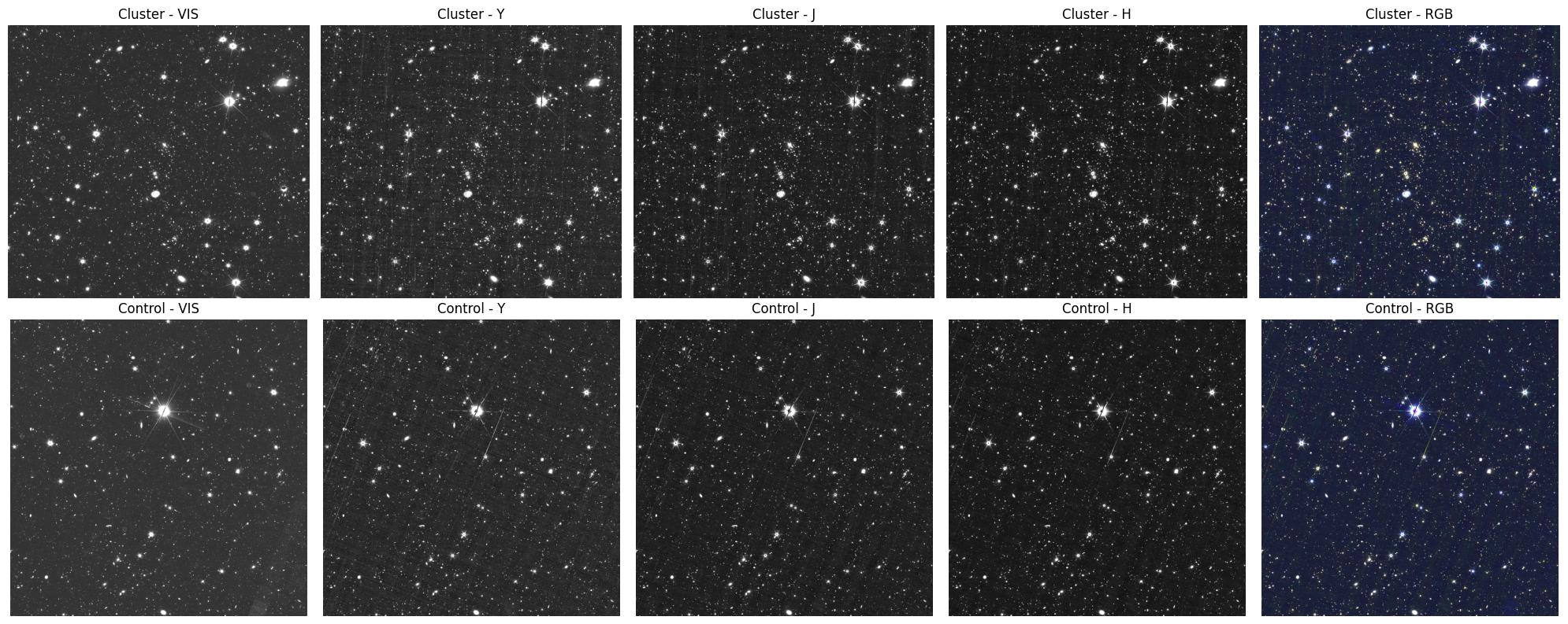
Figure 1. Euclid Q1 MER cutouts of the cluster candidate and control field. Top row: the cluster candidate field shown in the Euclid VIS band and the three NISP near-infrared bands (Y, J, H), followed by an RGB composite constructed as R = H, G = J, B = VIS. Bottom row: a nearby control field displayed in the same set of bands and with the same RGB mapping.
The images give a qualitative impression of the cluster, but to identify members and compare their properties we need the photometric catalog. We query the Euclid Q1 MER photometric catalog and the photometric redshift (photo-z) catalog from IRSA, joining them on object ID and filtering to galaxies at the cluster redshift with well-constrained photo-z uncertainties.
# Query galaxies in both fields with BOX search
table_mer = 'euclid_q1_mer_catalogue'
table_phz = 'euclid_q1_phz_photo_z'

# Convert cutout size to degrees
cutout_deg = im_cutout.to(u.deg).value
We now query both fields for galaxies that fall within a narrow photometric redshift slice centered on the cluster redshift (±0.12). Querying the same redshift slice in both the cluster and control fields is what makes the overdensity comparison meaningful. We do a cursory overdensity calculation based on the number of galaxies in the cluster field over number of galaxies in the control field identified in the redshift slice. Then we show part of the cluster dataframe to see what information we have available.
def query_galaxies_for_field(ra, dec, field_name, redshift_center, redshift_width=0.1):
    """Query galaxies within a redshift slice around a sky position.

    Submits a TAP/ADQL query to IRSA joining the Euclid Q1 MER photometric
    catalogue and the photo-z catalogue. Only objects satisfying all of the
    following criteria are returned:

    - Positive flux in all four bands (VIS, Y, J, H).
    - Photo-z classification = 2 (galaxy).
    - Fractional 90% credible interval width < 0.20, i.e.
      ``(phz_90_int2 - phz_90_int1) / (1 + phz_median) < 0.20``, selecting
      sources with well-constrained photometric redshifts.
    - ``phz_median`` within ``redshift_center ± redshift_width``.

    Parameters
    ----------
    ra : float
        Field centre RA in degrees.
    dec : float
        Field centre Dec in degrees.
    field_name : str
        Label used in progress messages.
    redshift_center : float
        Central photometric redshift of the cluster.
    redshift_width : float, optional
        Half-width of the redshift slice. Default is 0.1.

    Returns
    -------
    result : `~astropy.table.Table`
        Catalogue of galaxies matching all quality and spatial cuts.
    """
    print(f"\nQuerying galaxies for {field_name} field...")

    adql = (f"SELECT DISTINCT mer.object_id, mer.ra, mer.dec, "
            f"phz.flux_vis_unif, phz.flux_y_unif, phz.flux_j_unif, phz.flux_h_unif, "
            f"phz.phz_classification, phz.phz_median, phz.phz_90_int1, phz.phz_90_int2 "
            f"FROM {table_mer} AS mer "
            f"JOIN {table_phz} as phz "
            f"ON mer.object_id = phz.object_id "
            f"WHERE 1 = CONTAINS(POINT('ICRS', mer.ra, mer.dec), "
            f"BOX('ICRS', {ra}, {dec}, {cutout_deg/np.cos(np.radians(dec))}, {cutout_deg})) "
            f"AND phz.flux_vis_unif > 0 "
            f"AND phz.flux_y_unif > 0 "
            f"AND phz.flux_j_unif > 0 "
            f"AND phz.flux_h_unif > 0 "
            f"AND phz.phz_classification = 2 "
            f"AND ((phz.phz_90_int2 - phz.phz_90_int1) / (1 + phz.phz_median)) < 0.20 "
            f"AND phz.phz_median BETWEEN {redshift_center-redshift_width} AND {redshift_center+redshift_width}")

    result = Irsa.query_tap(adql).to_table()
    print(f"Found {len(result)} galaxies in {field_name} field (z = {redshift_center:.2f} ± {redshift_width:.2f})")

    return result
# Query galaxies for both fields in the cluster redshift slice
cluster_galaxies = query_galaxies_for_field(
cluster['RAPZWav'], cluster['DecPZWav'], "cluster",
cluster['zPZWav'], redshift_width=0.12
)
control_galaxies = query_galaxies_for_field(
control_ra, control_dec, "control",
cluster['zPZWav'], redshift_width=0.12
)
# Convert to pandas DataFrames for easier analysis
cluster_df_galaxies = cluster_galaxies.to_pandas()
control_df_galaxies = control_galaxies.to_pandas()
# Calculate Overdensity delta
n_cluster = len(cluster_galaxies)
n_control = len(control_galaxies)
# Avoid division by zero just in case
if n_control > 0:
overdensity = (n_cluster - n_control) / n_control
ratio = n_cluster / n_control
else:
overdensity = np.inf
ratio = np.inf
print(f"\nDensity Analysis:")
print(f"Cluster field: {n_cluster} galaxies")
print(f"Control field: {n_control} galaxies")
print(f"Density Ratio (N_clust/N_cont): {ratio:.2f}")
print(f"Measured Overdensity (delta): {overdensity:.2f}")
cluster_df_galaxies.head()
Querying galaxies for cluster field...
Found 704 galaxies in cluster field (z = 0.55 ± 0.12)

Querying galaxies for control field...
Found 216 galaxies in control field (z = 0.55 ± 0.12)

Density Analysis:
Cluster field: 704 galaxies
Control field: 216 galaxies
Density Ratio (N_clust/N_cont): 3.26
Measured Overdensity (delta): 2.26
5. Cluster Finding Algorithm
We apply DBSCAN (Density-Based Spatial Clustering of Applications with Noise) to the galaxy catalogues to confirm the cluster detection and identify candidate member galaxies. DBSCAN is well-suited to this problem because it finds arbitrarily shaped overdensities without requiring a prior on the number of clusters, and it naturally labels sparse galaxies as noise, useful for separating cluster members from the field population.
How redshift enters the analysis
Redshift is not an input to DBSCAN itself. Instead, both the cluster and control catalogues were already filtered in Section 4 to a narrow photo-z slice centred on the target cluster redshift (Δz = ±0.12). DBSCAN therefore operates on the projected 2-D sky distribution of galaxies. A real cluster should produce a compact spatial overdensity in this slice; the control field should show mostly noise.
Pixel coordinates vs. sky coordinates
Clustering is performed in image pixel space rather than in sky (RA/Dec) coordinates.
The main practical reason is that eps can be directly interpreted as an angular scale without computing a great-circle distance matrix.
At the native Euclid VIS pixel scale of ~0.1 arcsec/pixel, eps = 500 pixels corresponds to ~50 arcsec on the sky, and at z~0.4 this maps to roughly 300 kpc, comparable to the virial radius of a moderate-mass cluster.
This approach is accurate over the small field of view of a single 12-arcmin cutout where projection effects are negligible.
Parameter choices and customisation
The defaults eps=500 and min_samples=18 were tuned empirically for a 12-arcmin cutout at z~0.4 with Euclid Q1 data.
They are not universal, the right values depend on the cluster redshift, richness, cutout size, and the depth of the photo-z sample.
In particular:
The physical scale probed by
epschanges with redshift. At higher redshift the same angular scale subtends a larger physical distance, so you may want to increaseepsto keep the probed scale near the virial radius.min_samplessets the minimum richness threshold for a detection; increasing it suppresses spurious small groups, while decreasing it recovers lower-richness structures at the cost of more false positives.A more physically motivated approach is to convert the expected virial radius at the cluster redshift (in arcseconds) to pixels and use that as
eps.
Query/cutout mismatch and edge effects
The galaxy catalogue is queried with a rectangular BOX in ICRS coordinates, while the image cutout is defined in pixel space. Due to WCS projection distortions, a small fraction of galaxies returned by the query will map to pixel positions outside the image bounds and are excluded before clustering. If the cluster or control field is close to a tile edge, this fraction may be larger, reducing the effective sample size and potentially biasing results. The function prints the number of galaxies within bounds as a diagnostic, if a large fraction are lost, consider selecting a field better centred on the tile.
def apply_dbscan_clustering(galaxy_df, wcs, rgb_image, field_name, eps=500, min_samples=18):
    """Apply DBSCAN to detect galaxy overdensities in a redshift-selected sample. DBSCAN operates on the 2-D projected
    spatial distribution of galaxies at approximately the same redshift.

    **Parameter choices**

    ``eps=500`` and ``min_samples=18`` were tuned empirically for a 12-arcmin
    cutout at z~0.4 with a photo-z slice width of Δz=0.12. These values are
    data-dependent — feel free to adjust them to suit your science case:

    - Increase ``eps`` for higher-redshift or lower-richness clusters where
      members are more widely separated in projection.
    - Increase ``min_samples`` to suppress spurious small groups; decrease it
      to detect lower-richness structures.
    - For a physically motivated approach, estimate the virial radius at the
      cluster redshift, convert to pixels, and use that as ``eps``.

    Parameters
    ----------
    galaxy_df : `pandas.DataFrame`
        Galaxies pre-filtered to the cluster redshift slice, with columns
        ``ra`` and ``dec`` in degrees.
    wcs : `~astropy.wcs.WCS`
        WCS of the image cutout, used to project RA/Dec to pixel coordinates.
    rgb_image : `~numpy.ndarray`
        The RGB image array; its shape defines the valid pixel bounds.
    field_name : str
        Label used in printed diagnostics.
    eps : float, optional
        Maximum distance in pixels between neighbours in DBSCAN. Default is
        500 px (~50 arcsec at VIS resolution, ~300 kpc at z~0.4).
    min_samples : int, optional
        Minimum number of galaxies required to form a core point. Default is 18.

    Returns
    -------
    labels : `~numpy.ndarray`
        DBSCAN cluster labels for the valid galaxy subset; -1 indicates noise.
    valid_galaxy_coords : `~numpy.ndarray`
        (N, 2) pixel coordinate array for the galaxies that were clustered.
    n_clusters : int
        Number of clusters found (noise points excluded).
    n_noise : int
        Number of noise (unassigned) galaxies.
    """
    print(f"\nApplying DBSCAN clustering to {field_name} field...")

    # Convert galaxy coordinates to pixel coordinates
    galaxy_pixels = wcs.world_to_pixel_values(galaxy_df['ra'], galaxy_df['dec'])

    # Filter galaxies to only show those within the image bounds (needed due to query/cutout mismatch)
    image_height, image_width = rgb_image.shape[:2]
    valid_mask = ((galaxy_pixels[0] >= 0) & (galaxy_pixels[0] < image_width) &
                  (galaxy_pixels[1] >= 0) & (galaxy_pixels[1] < image_height))

    valid_galaxy_coords = np.column_stack([galaxy_pixels[0][valid_mask], galaxy_pixels[1][valid_mask]])

    print(f"  Total galaxies: {len(galaxy_df)}")
    print(f"  Galaxies within image bounds: {valid_mask.sum()}")

    # Apply DBSCAN clustering only to valid galaxies
    clustering = DBSCAN(eps=eps, min_samples=min_samples).fit(valid_galaxy_coords)
    labels = clustering.labels_

    # Count clusters (excluding noise points labeled as -1)
    n_clusters = len(set(labels)) - (1 if -1 in labels else 0)
    n_noise = list(labels).count(-1)

    print(f"{field_name} field: {n_clusters} clusters, {n_noise} noise points")

    return labels, valid_galaxy_coords, n_clusters, n_noise
A genuine cluster should produce a compact spatial overdensity in the redshift slice; the control field should show mostly noise. We run DBSCAN on both fields so we can compare the results directly.
# Apply clustering to both fields (with validity check)
cluster_labels, cluster_galaxy_coords, cluster_n_clusters, cluster_n_noise = apply_dbscan_clustering(
    cluster_df_galaxies, cluster_cutout_wcs, cluster_rgb, "Cluster"
)

control_labels, control_galaxy_coords, control_n_clusters, control_n_noise = apply_dbscan_clustering(
    control_df_galaxies, control_cutout_wcs, control_rgb, "Control"
)
Applying DBSCAN clustering to Cluster field...
  Total galaxies: 704
  Galaxies within image bounds: 500
Cluster field: 2 clusters, 269 noise points

Applying DBSCAN clustering to Control field...
  Total galaxies: 216
  Galaxies within image bounds: 195
Control field: 0 clusters, 195 noise points
# Plot clustering results for both fields in one figure (1 row, 2 columns)
fig, (ax1, ax2) = plt.subplots(1, 2, figsize=(20, 8),
                               subplot_kw={'projection': cluster_cutout_wcs})

# Cluster field (left subplot)
ax1.imshow(cluster_rgb, origin='lower')
if len(cluster_labels) > 0:
    cluster_unique_labels = set(cluster_labels)
    cluster_colors = plt.cm.Spectral(np.linspace(0, 1, len(cluster_unique_labels)))

    for k, col in zip(cluster_unique_labels, cluster_colors):
        if k == -1:
            continue  # noise points not shown
        class_member_mask = (cluster_labels == k)
        xy = cluster_galaxy_coords[class_member_mask]
        if len(xy) > 0:  # Check if there are any points to plot
            ax1.scatter(xy[:, 0], xy[:, 1], c=[col], marker='o', s=30, alpha=0.7)
else:
    print("No cluster data to plot")

ax1.set_xlabel('RA')
ax1.set_ylabel('Dec')
ax1.set_title(f'Cluster Field - {cluster_n_clusters} clusters')

# Control field (right subplot)
ax2.imshow(control_rgb, origin='lower')
if len(control_labels) > 0:
    control_unique_labels = set(control_labels)
    control_colors = plt.cm.Spectral(np.linspace(0, 1, len(control_unique_labels)))

    for k, col in zip(control_unique_labels, control_colors):
        if k == -1:
            continue  # noise points not shown
        class_member_mask = (control_labels == k)
        xy = control_galaxy_coords[class_member_mask]
        if len(xy) > 0:  # Check if there are any points to plot
            ax2.scatter(xy[:, 0], xy[:, 1], c=[col], marker='o', s=30, alpha=0.7)
else:
    print("No control field data to plot")

ax2.set_xlabel('RA')
ax2.set_ylabel('Dec')
ax2.set_title(f'Control Field - {control_n_clusters} clusters')

plt.tight_layout()
plt.show()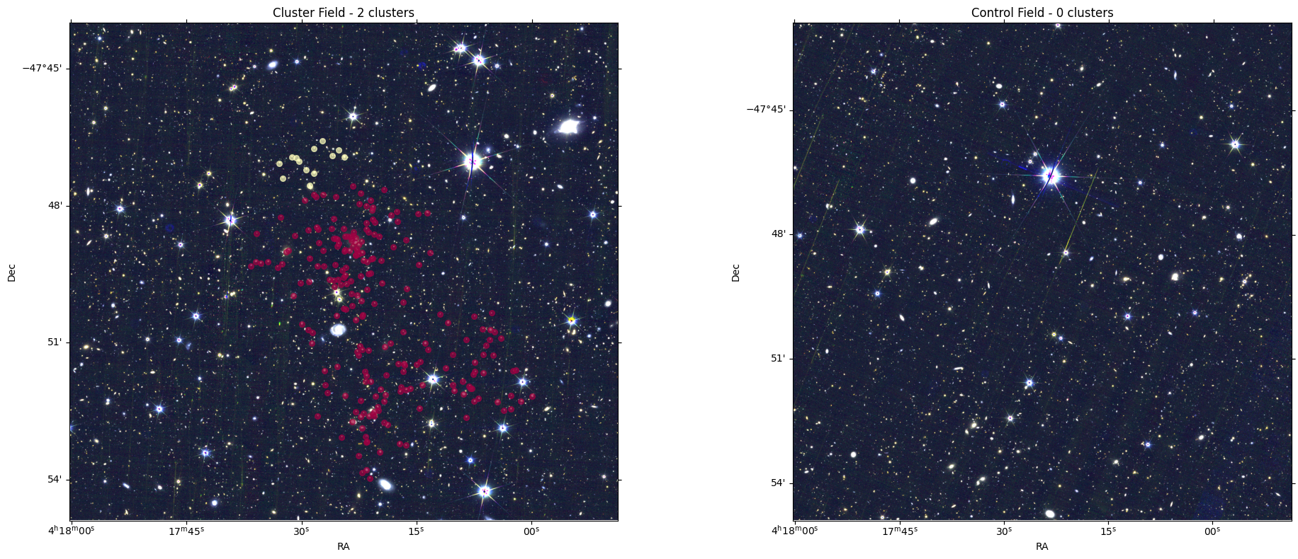
Figure 2. DBSCAN clustering of galaxy candidates in redshift slices: cluster field vs. control field. Each panel shows the RGB cutout (R = H, G = J, B = VIS) with points overplotted for sources selected within successive redshift slices and clustered using DBSCAN (density-based spatial clustering). Points assigned to a DBSCAN cluster are shown as colored circular markers; noise/outlier points (DBSCAN label = −1) are not shown. The left panel (cluster field) contains multiple spatial overdensities identified by DBSCAN, consistent with the expectation that a real cluster field may include one or more galaxy concentrations within the scanned redshift range. In the right panel (control field), no real clusters are found as expected. In some examples, a “cluster” can be identified around a bright star; this is interpreted as an artifact-driven detection (e.g., spurious sources near diffraction spikes/halos in Euclid Q1), rather than a genuine galaxy overdensity.
6. Color-Magnitude Diagram Analysis
We analyze the color-magnitude properties of cluster and field galaxies to understand their stellar populations and star formation histories. The Y-H color vs H magnitude diagram reveals differences in galaxy properties between cluster and field environments. With the DBSCAN labels computed, we separate each field’s galaxy catalog into cluster members (label ≥ 0) and field galaxies (label = −1). Combining field galaxies from both the cluster and control fields gives us a larger baseline sample for comparison.
def identify_cluster_members(galaxy_df, labels, galaxy_coords, field_name):
    """Separate a galaxy sample into cluster members and field galaxies.

    Re-applies the same image-bounds filter used in
    :func:`apply_dbscan_clustering` to align ``galaxy_df`` with the DBSCAN
    ``labels`` array, which only covers galaxies that fell within the image
    footprint. Galaxies with ``label != -1`` are cluster members; those with
    ``label == -1`` are noise (field galaxies).

    Parameters
    ----------
    galaxy_df : `pandas.DataFrame`
        Full galaxy catalogue for the field (before image-bounds filtering),
        with columns ``ra`` and ``dec`` in degrees.
    labels : `~numpy.ndarray`
        DBSCAN labels as returned by :func:`apply_dbscan_clustering`.
    galaxy_coords : `~numpy.ndarray`
        Pixel coordinates of the clustered galaxies (unused directly but kept
        for API consistency).
    field_name : str
        Either ``"Cluster"`` or ``"Control"``; selects the WCS and image used
        for the bounds filter.

    Returns
    -------
    cluster_members : `pandas.DataFrame`
        Galaxies assigned to a cluster group, with an added ``cluster_id``
        column containing the DBSCAN label.
    field_galaxies : `pandas.DataFrame`
        Galaxies classified as noise (``cluster_id = -1``).
    """
    print(f"\nAnalyzing {field_name} field galaxy populations...")

    # The labels array corresponds to the galaxies that were actually used in clustering
    # (those within image bounds). We need to create a mapping.

    # Get the WCS for coordinate conversion
    if field_name == "Cluster":
        wcs = cluster_cutout_wcs
        rgb_image = cluster_rgb
    else:
        wcs = control_cutout_wcs
        rgb_image = control_rgb

    # Convert galaxy coordinates to pixel coordinates
    galaxy_pixels = wcs.world_to_pixel_values(galaxy_df['ra'], galaxy_df['dec'])

    # Filter galaxies to only show those within the image bounds (same as in clustering)
    image_height, image_width = rgb_image.shape[:2]
    valid_mask = ((galaxy_pixels[0] >= 0) & (galaxy_pixels[0] < image_width) &
                  (galaxy_pixels[1] >= 0) & (galaxy_pixels[1] < image_height))

    # Get only the valid galaxies (those used in clustering)
    valid_galaxies = galaxy_df[valid_mask].copy()

    print(f"  Total galaxies in catalog: {len(galaxy_df)}")
    print(f"  Galaxies within image bounds: {len(valid_galaxies)}")
    print(f"  Labels array length: {len(labels)}")

    # Now the labels array should match the valid_galaxies DataFrame
    if len(valid_galaxies) != len(labels):
        print(f"  WARNING: Mismatch between valid galaxies ({len(valid_galaxies)}) and labels ({len(labels)})")
        # Use the minimum length to avoid errors
        min_len = min(len(valid_galaxies), len(labels))
        valid_galaxies = valid_galaxies.iloc[:min_len]
        labels = labels[:min_len]

    # Create a mask for cluster members (labels != -1)
    cluster_member_mask = labels != -1
    field_galaxy_mask = labels == -1

    # Get cluster members and field galaxies
    cluster_members = valid_galaxies[cluster_member_mask].copy()
    field_galaxies = valid_galaxies[field_galaxy_mask].copy()

    # Add cluster assignment information
    cluster_members['cluster_id'] = labels[cluster_member_mask]
    field_galaxies['cluster_id'] = -1  # Field galaxies

    print(f"  Cluster members: {len(cluster_members)} galaxies")
    print(f"  Field galaxies: {len(field_galaxies)} galaxies")

    # Count galaxies per cluster
    if len(cluster_members) > 0:
        cluster_counts = cluster_members['cluster_id'].value_counts().sort_index()

    return cluster_members, field_galaxies
# Analyze both fields
cluster_members_cluster_field, field_galaxies_cluster_field = identify_cluster_members(
cluster_df_galaxies, cluster_labels, cluster_galaxy_coords, "Cluster"
)
cluster_members_control_field, field_galaxies_control_field = identify_cluster_members(
control_df_galaxies, control_labels, control_galaxy_coords, "Control"
)
# Combine all field galaxies (from both cluster and control fields)
all_field_galaxies = pd.concat([field_galaxies_cluster_field, field_galaxies_control_field], ignore_index=True)
# Combine all cluster members
all_cluster_members = pd.concat([cluster_members_cluster_field], ignore_index=True)
print(f"\nOverall Summary:")
print(f"Total cluster members: {len(all_cluster_members)}")
print(f"Total field galaxies: {len(all_field_galaxies)}")
Analyzing Cluster field galaxy populations...
  Total galaxies in catalog: 704
  Galaxies within image bounds: 500
  Labels array length: 500
  Cluster members: 231 galaxies
  Field galaxies: 269 galaxies

Analyzing Control field galaxy populations...
  Total galaxies in catalog: 216
  Galaxies within image bounds: 195
  Labels array length: 195
  Cluster members: 0 galaxies
  Field galaxies: 195 galaxies

Overall Summary:
Total cluster members: 231
Total field galaxies: 464
At z~0.4, the H band probes rest-frame near-infrared light dominated by old, low-mass stars, while the Y band samples shorter wavelengths where younger stellar populations contribute more. The Y−H color therefore tracks the age and star formation activity of the stellar population. Passive ellipticals galaxies in a cluster at the same redshift, that have stopped forming stars, tend to share similar Y−H colors, producing a tight sequence in the color-magnitude diagram known as the red sequence. We convert the uniform-aperture fluxes in the photo-z catalog to AB magnitudes and exclude objects outside physically reasonable bounds (H < 17 or H > 25, or |Y−H| outside [−0.5, 1.5]) to remove saturated sources, noise-dominated detections, and photometric outliers.
def calculate_color_magnitude(df):
    """Convert uniform-aperture fluxes to AB magnitudes and compute Y-H color.

    Magnitudes are computed as ``m = -2.5 * log10(flux) + 23.9``, where the
    zero-point 23.9 corresponds to fluxes in microjanskies — the unit of the
    ``flux_*_unif`` columns in the Euclid Q1 photo-z catalogue. The resulting
    magnitudes are not K-corrected or corrected for Milky Way extinction.

    Parameters
    ----------
    df : `pandas.DataFrame`
        DataFrame containing columns ``flux_y_unif`` and ``flux_h_unif`` in
        microjanskies. Both must be positive (no non-detections).

    Returns
    -------
    df : `pandas.DataFrame`
        Copy of the input with three additional columns: ``H_mag``, ``Y_mag``
        (AB magnitudes), and ``Y_H_color``.
    """
    df = df.copy()

    # Convert fluxes to magnitudes (using -2.5 * log10(flux))
    # Note: These are instrumental magnitudes, not absolute magnitudes
    df['H_mag'] = -2.5 * np.log10(df['flux_h_unif'])+23.9
    df['Y_mag'] = -2.5 * np.log10(df['flux_y_unif'])+23.9

    # Calculate Y-H color
    df['Y_H_color'] = df['Y_mag'] - df['H_mag']

    return df
# Calculate color-magnitude properties using only the needed fluxes
cluster_cmd = calculate_color_magnitude(all_cluster_members[['flux_y_unif', 'flux_h_unif']])
field_cmd = calculate_color_magnitude(all_field_galaxies[['flux_y_unif', 'flux_h_unif']])def remove_outliers_bounds(df, h_min=17, h_max=25, yh_min=-0.5, yh_max=1.5):
"""Filter a colour-magnitude table to a physically motivated range.
Retains only rows whose H-band magnitude and Y-H colour fall within the
specified boundaries. The defaults bracket the expected locus of cluster
galaxies at z~0.4 in Euclid Q1 data: objects brighter than H=17 are likely
stars or saturated; objects fainter than H=25 have unreliable photo-z and
colours; Y-H outside [-0.5, 1.5] typically indicates bad photometry or
non-galaxy contaminants.
Parameters
----------
df : `pandas.DataFrame`
DataFrame with columns ``H_mag`` and ``Y_H_color``.
h_min : float, optional
Minimum H magnitude (brightest limit). Default is 17.
h_max : float, optional
Maximum H magnitude (faintest limit). Default is 25.
yh_min : float, optional
Minimum Y-H colour. Default is -0.5.
yh_max : float, optional
Maximum Y-H colour. Default is 1.5.
Returns
-------
df_clean : `pandas.DataFrame`
Filtered copy of the input DataFrame.
"""
df_clean = df.copy()
df_clean = df_clean[
(df_clean['H_mag'] >= h_min) & (df_clean['H_mag'] <= h_max) &
(df_clean['Y_H_color'] >= yh_min) & (df_clean['Y_H_color'] <= yh_max)
]
return df_clean# Remove outliers from both populations (using plot boundaries)
print("Removing outliers outside plot boundaries...")
cluster_cmd_clean = remove_outliers_bounds(cluster_cmd)
field_cmd_clean = remove_outliers_bounds(field_cmd)
print(f"Cluster galaxies: {len(cluster_cmd)} -> {len(cluster_cmd_clean)} (removed {len(cluster_cmd) - len(cluster_cmd_clean)})")
print(f"Field galaxies: {len(field_cmd)} -> {len(field_cmd_clean)} (removed {len(field_cmd) - len(field_cmd_clean)})")Removing outliers outside plot boundaries...
Cluster galaxies: 231 -> 229 (removed 2)
Field galaxies: 464 -> 454 (removed 10)
fig, ax = plt.subplots(1, 1, figsize=(8, 5))

# Plot comparison with lower alpha for better visibility
ax.scatter(field_cmd_clean['H_mag'], field_cmd_clean['Y_H_color'],
          c='blue', alpha=0.1, s=25, label=f'Field ({len(field_cmd_clean)})')
ax.scatter(cluster_cmd_clean['H_mag'], cluster_cmd_clean['Y_H_color'],
          c='red', alpha=0.1, s=30, label=f'Cluster ({len(cluster_cmd_clean)})')

# Add density contours to show the tightness of each population

# Create density contours for field galaxies (using cleaned data)
if len(field_cmd_clean) > 10:  # Need enough points for meaningful contours
    field_h = field_cmd_clean['H_mag'].values
    field_yh = field_cmd_clean['Y_H_color'].values
    field_xy = np.vstack([field_h, field_yh])
    field_density = gaussian_kde(field_xy)

    # Create grid for contour plot
    h_grid = np.linspace(17, 25, 100)
    yh_grid = np.linspace(-0.5, 1.5, 100)
    H_grid, YH_grid = np.meshgrid(h_grid, yh_grid)
    positions = np.vstack([H_grid.ravel(), YH_grid.ravel()])
    field_z = np.reshape(field_density(positions).T, H_grid.shape)

    # Plot field contours
    ax.contour(H_grid, YH_grid, field_z, levels=3, colors='blue', alpha=0.6, linestyles='--', linewidths=1)

# Create density contours for cluster galaxies (using cleaned data)
if len(cluster_cmd_clean) > 10:  # Need enough points for meaningful contours
    cluster_h = cluster_cmd_clean['H_mag'].values
    cluster_yh = cluster_cmd_clean['Y_H_color'].values
    cluster_xy = np.vstack([cluster_h, cluster_yh])
    cluster_density = gaussian_kde(cluster_xy)

    # Use same grid
    cluster_z = np.reshape(cluster_density(positions).T, H_grid.shape)

    # Plot cluster contours
    ax.contour(H_grid, YH_grid, cluster_z, levels=3, colors='red', alpha=0.8, linestyles='-', linewidths=2)

ax.set_xlabel('H Magnitude')
ax.set_ylabel('Y-H Color')
ax.set_title('Cluster vs Field Color-Magnitude Diagram\n(with density contours)')
ax.grid(True, alpha=0.3)
ax.legend()

# Set axis limits as requested
ax.set_xlim(17, 25)  # H magnitude range
ax.set_ylim(-0.5, 1.5)  # Y-H color range

plt.tight_layout()
plt.show()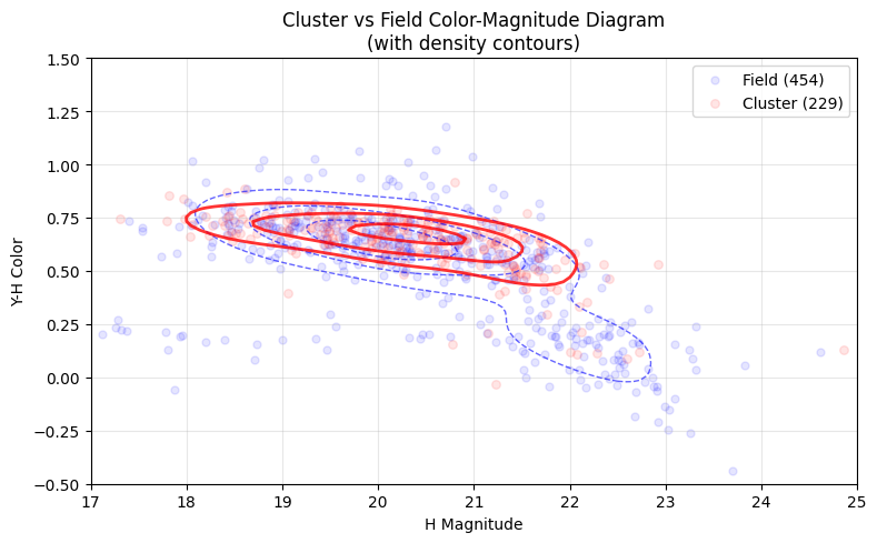
Figure 3. Y−H versus H colour–magnitude diagram for the cluster candidates compared to the control field.
We construct an H-band magnitude and a Y−H colour from the Euclid Q1 uniform-aperture fluxes (flux_h_unif, flux_y_unif) by converting microjansky fluxes to AB magnitudes.
Points show individual objects: cluster members (red) and field galaxies (blue).
To highlight the dominant loci beyond the sparse scatter, we overlay density contours derived from a 2D Gaussian kernel density estimate (KDE) computed in the ((H,,Y-H)) plane separately for the cluster and field samples. The KDE is evaluated on a regular grid spanning the plotted limits, and three contour levels are drawn for each population (solid red for cluster; dashed blue for field). A genuine cluster is expected to show a relatively tighter and/or shifted colour–magnitude locus compared to the general field population (e.g., a concentration consistent with a red-sequence-like population), while the field sample traces the broader distribution of galaxies along the line of sight.
7. Spectral Analysis
Euclid’s NISP instrument provides slitless near-infrared spectra covering roughly 9,200–18,800 Å. At the cluster redshift of z~0.55, common optical emission lines — Hα (6563 Å), [OII] (3727 Å), [OIII] (5007 Å), are redshifted into this wavelength window. Active star-forming galaxies show strong emission in these lines while passive (quiescent) galaxies do not, so comparing the median spectra of cluster members versus field galaxies can reveal whether the dense cluster environment has suppressed star formation.
The analysis continuum-subtracts each spectrum, normalizes it to a common scale, and marks the expected observed wavelengths of emission lines at the cluster redshift.
Note: This section is computationally intensive and may be skipped for an initial look at the data.
spectra_cache_dir = "data/irsa_spectra"
os.makedirs(spectra_cache_dir, exist_ok=True)

BUCKET_NAME = "nasa-irsa-euclid-q1"
table_1dspectra = "euclid.objectid_spectrafile_association_q1"

cluster_object_ids = all_cluster_members["object_id"].tolist()
field_object_ids   = all_field_galaxies["object_id"].tolist()
We retrieve up to ten spectra for each population. Ten spectra per group is sufficient to show whether the cluster and field populations differ in their emission-line properties.
def get_n_spectra(obj_ids, n=10):
    """
    Fetch up to n spectra for the given object_ids, stopping early once n are found.
    Uses one TAP query, groups by FITS file, caches per-object results in ./data/irsa_spectra/.
    Skips TAP rows with missing (masked) HDU indices.
    """
    obj_ids = [int(x) for x in obj_ids]
    if len(obj_ids) == 0 or n <= 0:
        return {}

    # Cache-first
    spectra = {}
    remaining = []
    for oid in obj_ids:
        cache_npz = os.path.join(spectra_cache_dir, f"{oid}.npz")
        if os.path.exists(cache_npz):
            d = np.load(cache_npz)
            spectra[oid] = {
                "wave": d["wave"] * u.angstrom,
                "flux": d["flux"] * (u.erg / u.s / u.cm**2 / u.angstrom),
                "error": d["error"] * (u.erg / u.s / u.cm**2 / u.angstrom),
                "object_id": oid,
            }
            if len(spectra) >= n:
                return dict(list(spectra.items())[:n])
        else:
            remaining.append(oid)

    if len(remaining) == 0:
        return dict(list(spectra.items())[:n])

    # TAP query once
    id_list = ",".join(map(str, remaining))
    adql_query = f"""
    SELECT objectid, path, hdu
    FROM {table_1dspectra}
    WHERE objectid IN ({id_list})
    """

    try:
        assoc = Irsa.query_tap(adql_query).to_table()
    except (DALQueryError, requests.exceptions.RequestException) as e:
        print("TAP query failed:", e)
        return dict(list(spectra.items())[:n])

    if len(assoc) == 0:
        print("No spectrum associations returned.")
        return dict(list(spectra.items())[:n])

    # Group by FITS file, skipping masked/invalid hdu
    groups = {}
    skipped_hdu = 0

    for row in assoc:
        obj_id = int(row["objectid"])
        uri = str(row["path"])

        # HDU can be masked for some rows -> skip
        hdu_val = row["hdu"]
        try:
            # This will fail for masked values
            hdu_index = int(hdu_val)
        except Exception:
            skipped_hdu += 1
            continue

        spec_fpath_key = uri.replace("api/spectrumdm/convert/euclid/", "").split("?")[0]
        s3_uri = f"s3://{BUCKET_NAME}/{spec_fpath_key}"
        groups.setdefault(s3_uri, []).append((obj_id, hdu_index))

    if skipped_hdu > 0:
        print(f"Skipped {skipped_hdu} TAP rows with missing/invalid HDU indices.")

    if len(groups) == 0:
        print("No usable (path,hdu) associations after filtering.")
        return dict(list(spectra.items())[:n])

    # Open files with progress bar
    for s3_uri, items in tqdm(list(groups.items()), desc="Opening FITS files", unit="file"):
        if len(spectra) >= n:
            break

        try:
            with fits.open(s3_uri, fsspec_kwargs={"anon": True}, lazy_load_hdus=True) as hdul:
                for (obj_id, hdu_index) in items:
                    if len(spectra) >= n:
                        break

                    try:
                        spec = QTable.read(hdul[hdu_index], format="fits")
                        header = hdul[hdu_index].header

                        fscale = header.get("FSCALE", 1.0)
                        wave = np.asarray(spec["WAVELENGTH"]) * u.angstrom
                        signal = np.asarray(spec["SIGNAL"])
                        var = np.asarray(spec["VAR"])
                        mask = np.asarray(spec["MASK"])

                        if not (len(wave) == len(signal) == len(var) == len(mask)):
                            continue

                        valid = (mask % 2 == 0) & (mask < 64)
                        wave = wave[valid]
                        flux = signal[valid] * fscale * u.erg / u.s / u.cm**2 / u.angstrom
                        error = np.sqrt(var[valid]) * fscale * flux.unit

                        spectra[obj_id] = {
                            "wave": wave,
                            "flux": flux,
                            "error": error,
                            "object_id": obj_id,
                        }

                        np.savez(
                            os.path.join(spectra_cache_dir, f"{obj_id}.npz"),
                            wave=wave.value,
                            flux=flux.value,
                            error=error.value,
                        )

                    except Exception:
                        continue

        except Exception as e:
            print(f"Failed to open {s3_uri}: {e}")
            continue

    return dict(list(spectra.items())[:n])
# Run (it will stop as soon as it finds 10 real spectra)
cluster_spectra = get_n_spectra(cluster_object_ids, n=10)
field_spectra = get_n_spectra(field_object_ids, n=10)
print(f"Cluster spectra retrieved: {len(cluster_spectra)}")
print(f"Field spectra retrieved: {len(field_spectra)}")
print(f"Cache dir: {spectra_cache_dir}/")Skipped 5 TAP rows with missing/invalid HDU indices.
Opening FITS files: 0%| | 0/24 [00:00<?, ?file/s]WARNING: UnitsWarning: 'Number' did not parse as fits unit: At col 0, Unit 'Number' not supported by the FITS standard. If this is meant to be a custom unit, define it with 'u.def_unit'. To have it recognized inside a file reader or other code, enable it with 'u.add_enabled_units'. For details, see https://docs.astropy.org/en/latest/units/combining_and_defining.html [astropy.units.core]
WARNING: UnitsWarning: 'Number' did not parse as fits unit: At col 0, Unit 'Number' not supported by the FITS standard.  If this is meant to be a custom unit, define it with 'u.def_unit'. To have it recognized inside a file reader or other code, enable it with 'u.add_enabled_units'. For details, see https://docs.astropy.org/en/latest/units/combining_and_defining.html [astropy.units.core]
WARNING: UnitsWarning: 'Number' did not parse as fits unit: At col 0, Unit 'Number' not supported by the FITS standard.  If this is meant to be a custom unit, define it with 'u.def_unit'. To have it recognized inside a file reader or other code, enable it with 'u.add_enabled_units'. For details, see https://docs.astropy.org/en/latest/units/combining_and_defining.html [astropy.units.core]
WARNING: UnitsWarning: 'Number' did not parse as fits unit: At col 0, Unit 'Number' not supported by the FITS standard.  If this is meant to be a custom unit, define it with 'u.def_unit'. To have it recognized inside a file reader or other code, enable it with 'u.add_enabled_units'. For details, see https://docs.astropy.org/en/latest/units/combining_and_defining.html [astropy.units.core]
WARNING: UnitsWarning: 'Number' did not parse as fits unit: At col 0, Unit 'Number' not supported by the FITS standard.  If this is meant to be a custom unit, define it with 'u.def_unit'. To have it recognized inside a file reader or other code, enable it with 'u.add_enabled_units'. For details, see https://docs.astropy.org/en/latest/units/combining_and_defining.html [astropy.units.core]
WARNING: UnitsWarning: 'Number' did not parse as fits unit: At col 0, Unit 'Number' not supported by the FITS standard.  If this is meant to be a custom unit, define it with 'u.def_unit'. To have it recognized inside a file reader or other code, enable it with 'u.add_enabled_units'. For details, see https://docs.astropy.org/en/latest/units/combining_and_defining.html [astropy.units.core]
WARNING: UnitsWarning: 'Number' did not parse as fits unit: At col 0, Unit 'Number' not supported by the FITS standard.  If this is meant to be a custom unit, define it with 'u.def_unit'. To have it recognized inside a file reader or other code, enable it with 'u.add_enabled_units'. For details, see https://docs.astropy.org/en/latest/units/combining_and_defining.html [astropy.units.core]
WARNING: UnitsWarning: 'Number' did not parse as fits unit: At col 0, Unit 'Number' not supported by the FITS standard.  If this is meant to be a custom unit, define it with 'u.def_unit'. To have it recognized inside a file reader or other code, enable it with 'u.add_enabled_units'. For details, see https://docs.astropy.org/en/latest/units/combining_and_defining.html [astropy.units.core]
WARNING: UnitsWarning: 'Number' did not parse as fits unit: At col 0, Unit 'Number' not supported by the FITS standard.  If this is meant to be a custom unit, define it with 'u.def_unit'. To have it recognized inside a file reader or other code, enable it with 'u.add_enabled_units'. For details, see https://docs.astropy.org/en/latest/units/combining_and_defining.html [astropy.units.core]
WARNING: UnitsWarning: 'Number' did not parse as fits unit: At col 0, Unit 'Number' not supported by the FITS standard.  If this is meant to be a custom unit, define it with 'u.def_unit'. To have it recognized inside a file reader or other code, enable it with 'u.add_enabled_units'. For details, see https://docs.astropy.org/en/latest/units/combining_and_defining.html [astropy.units.core]
WARNING: UnitsWarning: 'Number' did not parse as fits unit: At col 0, Unit 'Number' not supported by the FITS standard.  If this is meant to be a custom unit, define it with 'u.def_unit'. To have it recognized inside a file reader or other code, enable it with 'u.add_enabled_units'. For details, see https://docs.astropy.org/en/latest/units/combining_and_defining.html [astropy.units.core]
WARNING: UnitsWarning: 'Number' did not parse as fits unit: At col 0, Unit 'Number' not supported by the FITS standard.  If this is meant to be a custom unit, define it with 'u.def_unit'. To have it recognized inside a file reader or other code, enable it with 'u.add_enabled_units'. For details, see https://docs.astropy.org/en/latest/units/combining_and_defining.html [astropy.units.core]
WARNING: UnitsWarning: 'Number' did not parse as fits unit: At col 0, Unit 'Number' not supported by the FITS standard.  If this is meant to be a custom unit, define it with 'u.def_unit'. To have it recognized inside a file reader or other code, enable it with 'u.add_enabled_units'. For details, see https://docs.astropy.org/en/latest/units/combining_and_defining.html [astropy.units.core]
WARNING: UnitsWarning: 'Number' did not parse as fits unit: At col 0, Unit 'Number' not supported by the FITS standard.  If this is meant to be a custom unit, define it with 'u.def_unit'. To have it recognized inside a file reader or other code, enable it with 'u.add_enabled_units'. For details, see https://docs.astropy.org/en/latest/units/combining_and_defining.html [astropy.units.core]
WARNING: UnitsWarning: 'Number' did not parse as fits unit: At col 0, Unit 'Number' not supported by the FITS standard.  If this is meant to be a custom unit, define it with 'u.def_unit'. To have it recognized inside a file reader or other code, enable it with 'u.add_enabled_units'. For details, see https://docs.astropy.org/en/latest/units/combining_and_defining.html [astropy.units.core]
WARNING: UnitsWarning: 'Number' did not parse as fits unit: At col 0, Unit 'Number' not supported by the FITS standard.  If this is meant to be a custom unit, define it with 'u.def_unit'. To have it recognized inside a file reader or other code, enable it with 'u.add_enabled_units'. For details, see https://docs.astropy.org/en/latest/units/combining_and_defining.html [astropy.units.core]
WARNING: UnitsWarning: 'Number' did not parse as fits unit: At col 0, Unit 'Number' not supported by the FITS standard.  If this is meant to be a custom unit, define it with 'u.def_unit'. To have it recognized inside a file reader or other code, enable it with 'u.add_enabled_units'. For details, see https://docs.astropy.org/en/latest/units/combining_and_defining.html [astropy.units.core]
WARNING: UnitsWarning: 'Number' did not parse as fits unit: At col 0, Unit 'Number' not supported by the FITS standard.  If this is meant to be a custom unit, define it with 'u.def_unit'. To have it recognized inside a file reader or other code, enable it with 'u.add_enabled_units'. For details, see https://docs.astropy.org/en/latest/units/combining_and_defining.html [astropy.units.core]
WARNING: UnitsWarning: 'Number' did not parse as fits unit: At col 0, Unit 'Number' not supported by the FITS standard.  If this is meant to be a custom unit, define it with 'u.def_unit'. To have it recognized inside a file reader or other code, enable it with 'u.add_enabled_units'. For details, see https://docs.astropy.org/en/latest/units/combining_and_defining.html [astropy.units.core]
WARNING: UnitsWarning: 'Number' did not parse as fits unit: At col 0, Unit 'Number' not supported by the FITS standard.  If this is meant to be a custom unit, define it with 'u.def_unit'. To have it recognized inside a file reader or other code, enable it with 'u.add_enabled_units'. For details, see https://docs.astropy.org/en/latest/units/combining_and_defining.html [astropy.units.core]
WARNING: UnitsWarning: 'Number' did not parse as fits unit: At col 0, Unit 'Number' not supported by the FITS standard.  If this is meant to be a custom unit, define it with 'u.def_unit'. To have it recognized inside a file reader or other code, enable it with 'u.add_enabled_units'. For details, see https://docs.astropy.org/en/latest/units/combining_and_defining.html [astropy.units.core]
WARNING: UnitsWarning: 'Number' did not parse as fits unit: At col 0, Unit 'Number' not supported by the FITS standard.  If this is meant to be a custom unit, define it with 'u.def_unit'. To have it recognized inside a file reader or other code, enable it with 'u.add_enabled_units'. For details, see https://docs.astropy.org/en/latest/units/combining_and_defining.html [astropy.units.core]
WARNING: UnitsWarning: 'Number' did not parse as fits unit: At col 0, Unit 'Number' not supported by the FITS standard.  If this is meant to be a custom unit, define it with 'u.def_unit'. To have it recognized inside a file reader or other code, enable it with 'u.add_enabled_units'. For details, see https://docs.astropy.org/en/latest/units/combining_and_defining.html [astropy.units.core]
WARNING: UnitsWarning: 'Number' did not parse as fits unit: At col 0, Unit 'Number' not supported by the FITS standard.  If this is meant to be a custom unit, define it with 'u.def_unit'. To have it recognized inside a file reader or other code, enable it with 'u.add_enabled_units'. For details, see https://docs.astropy.org/en/latest/units/combining_and_defining.html [astropy.units.core]
WARNING: UnitsWarning: 'Number' did not parse as fits unit: At col 0, Unit 'Number' not supported by the FITS standard.  If this is meant to be a custom unit, define it with 'u.def_unit'. To have it recognized inside a file reader or other code, enable it with 'u.add_enabled_units'. For details, see https://docs.astropy.org/en/latest/units/combining_and_defining.html [astropy.units.core]
WARNING: UnitsWarning: 'Number' did not parse as fits unit: At col 0, Unit 'Number' not supported by the FITS standard.  If this is meant to be a custom unit, define it with 'u.def_unit'. To have it recognized inside a file reader or other code, enable it with 'u.add_enabled_units'. For details, see https://docs.astropy.org/en/latest/units/combining_and_defining.html [astropy.units.core]
WARNING: UnitsWarning: 'Number' did not parse as fits unit: At col 0, Unit 'Number' not supported by the FITS standard.  If this is meant to be a custom unit, define it with 'u.def_unit'. To have it recognized inside a file reader or other code, enable it with 'u.add_enabled_units'. For details, see https://docs.astropy.org/en/latest/units/combining_and_defining.html [astropy.units.core]
WARNING: UnitsWarning: 'Number' did not parse as fits unit: At col 0, Unit 'Number' not supported by the FITS standard.  If this is meant to be a custom unit, define it with 'u.def_unit'. To have it recognized inside a file reader or other code, enable it with 'u.add_enabled_units'. For details, see https://docs.astropy.org/en/latest/units/combining_and_defining.html [astropy.units.core]
WARNING: UnitsWarning: 'Number' did not parse as fits unit: At col 0, Unit 'Number' not supported by the FITS standard.  If this is meant to be a custom unit, define it with 'u.def_unit'. To have it recognized inside a file reader or other code, enable it with 'u.add_enabled_units'. For details, see https://docs.astropy.org/en/latest/units/combining_and_defining.html [astropy.units.core]
WARNING: UnitsWarning: 'Number' did not parse as fits unit: At col 0, Unit 'Number' not supported by the FITS standard.  If this is meant to be a custom unit, define it with 'u.def_unit'. To have it recognized inside a file reader or other code, enable it with 'u.add_enabled_units'. For details, see https://docs.astropy.org/en/latest/units/combining_and_defining.html [astropy.units.core]
Opening FITS files: 4%|▍ | 1/24 [00:02<00:56, 2.46s/file]Opening FITS files: 4%|▍ | 1/24 [00:02<00:56, 2.46s/file]
Skipped 38 TAP rows with missing/invalid HDU indices.
Opening FITS files: 0%| | 0/62 [00:00<?, ?file/s]WARNING: UnitsWarning: 'Number' did not parse as fits unit: At col 0, Unit 'Number' not supported by the FITS standard. If this is meant to be a custom unit, define it with 'u.def_unit'. To have it recognized inside a file reader or other code, enable it with 'u.add_enabled_units'. For details, see https://docs.astropy.org/en/latest/units/combining_and_defining.html [astropy.units.core]
WARNING: UnitsWarning: 'Number' did not parse as fits unit: At col 0, Unit 'Number' not supported by the FITS standard.  If this is meant to be a custom unit, define it with 'u.def_unit'. To have it recognized inside a file reader or other code, enable it with 'u.add_enabled_units'. For details, see https://docs.astropy.org/en/latest/units/combining_and_defining.html [astropy.units.core]
WARNING: UnitsWarning: 'Number' did not parse as fits unit: At col 0, Unit 'Number' not supported by the FITS standard.  If this is meant to be a custom unit, define it with 'u.def_unit'. To have it recognized inside a file reader or other code, enable it with 'u.add_enabled_units'. For details, see https://docs.astropy.org/en/latest/units/combining_and_defining.html [astropy.units.core]
WARNING: UnitsWarning: 'Number' did not parse as fits unit: At col 0, Unit 'Number' not supported by the FITS standard.  If this is meant to be a custom unit, define it with 'u.def_unit'. To have it recognized inside a file reader or other code, enable it with 'u.add_enabled_units'. For details, see https://docs.astropy.org/en/latest/units/combining_and_defining.html [astropy.units.core]
WARNING: UnitsWarning: 'Number' did not parse as fits unit: At col 0, Unit 'Number' not supported by the FITS standard.  If this is meant to be a custom unit, define it with 'u.def_unit'. To have it recognized inside a file reader or other code, enable it with 'u.add_enabled_units'. For details, see https://docs.astropy.org/en/latest/units/combining_and_defining.html [astropy.units.core]
WARNING: UnitsWarning: 'Number' did not parse as fits unit: At col 0, Unit 'Number' not supported by the FITS standard.  If this is meant to be a custom unit, define it with 'u.def_unit'. To have it recognized inside a file reader or other code, enable it with 'u.add_enabled_units'. For details, see https://docs.astropy.org/en/latest/units/combining_and_defining.html [astropy.units.core]
WARNING: UnitsWarning: 'Number' did not parse as fits unit: At col 0, Unit 'Number' not supported by the FITS standard.  If this is meant to be a custom unit, define it with 'u.def_unit'. To have it recognized inside a file reader or other code, enable it with 'u.add_enabled_units'. For details, see https://docs.astropy.org/en/latest/units/combining_and_defining.html [astropy.units.core]
WARNING: UnitsWarning: 'Number' did not parse as fits unit: At col 0, Unit 'Number' not supported by the FITS standard.  If this is meant to be a custom unit, define it with 'u.def_unit'. To have it recognized inside a file reader or other code, enable it with 'u.add_enabled_units'. For details, see https://docs.astropy.org/en/latest/units/combining_and_defining.html [astropy.units.core]
WARNING: UnitsWarning: 'Number' did not parse as fits unit: At col 0, Unit 'Number' not supported by the FITS standard.  If this is meant to be a custom unit, define it with 'u.def_unit'. To have it recognized inside a file reader or other code, enable it with 'u.add_enabled_units'. For details, see https://docs.astropy.org/en/latest/units/combining_and_defining.html [astropy.units.core]
WARNING: UnitsWarning: 'Number' did not parse as fits unit: At col 0, Unit 'Number' not supported by the FITS standard.  If this is meant to be a custom unit, define it with 'u.def_unit'. To have it recognized inside a file reader or other code, enable it with 'u.add_enabled_units'. For details, see https://docs.astropy.org/en/latest/units/combining_and_defining.html [astropy.units.core]
WARNING: UnitsWarning: 'Number' did not parse as fits unit: At col 0, Unit 'Number' not supported by the FITS standard.  If this is meant to be a custom unit, define it with 'u.def_unit'. To have it recognized inside a file reader or other code, enable it with 'u.add_enabled_units'. For details, see https://docs.astropy.org/en/latest/units/combining_and_defining.html [astropy.units.core]
WARNING: UnitsWarning: 'Number' did not parse as fits unit: At col 0, Unit 'Number' not supported by the FITS standard.  If this is meant to be a custom unit, define it with 'u.def_unit'. To have it recognized inside a file reader or other code, enable it with 'u.add_enabled_units'. For details, see https://docs.astropy.org/en/latest/units/combining_and_defining.html [astropy.units.core]
WARNING: UnitsWarning: 'Number' did not parse as fits unit: At col 0, Unit 'Number' not supported by the FITS standard.  If this is meant to be a custom unit, define it with 'u.def_unit'. To have it recognized inside a file reader or other code, enable it with 'u.add_enabled_units'. For details, see https://docs.astropy.org/en/latest/units/combining_and_defining.html [astropy.units.core]
WARNING: UnitsWarning: 'Number' did not parse as fits unit: At col 0, Unit 'Number' not supported by the FITS standard.  If this is meant to be a custom unit, define it with 'u.def_unit'. To have it recognized inside a file reader or other code, enable it with 'u.add_enabled_units'. For details, see https://docs.astropy.org/en/latest/units/combining_and_defining.html [astropy.units.core]
WARNING: UnitsWarning: 'Number' did not parse as fits unit: At col 0, Unit 'Number' not supported by the FITS standard.  If this is meant to be a custom unit, define it with 'u.def_unit'. To have it recognized inside a file reader or other code, enable it with 'u.add_enabled_units'. For details, see https://docs.astropy.org/en/latest/units/combining_and_defining.html [astropy.units.core]
WARNING: UnitsWarning: 'Number' did not parse as fits unit: At col 0, Unit 'Number' not supported by the FITS standard.  If this is meant to be a custom unit, define it with 'u.def_unit'. To have it recognized inside a file reader or other code, enable it with 'u.add_enabled_units'. For details, see https://docs.astropy.org/en/latest/units/combining_and_defining.html [astropy.units.core]
WARNING: UnitsWarning: 'Number' did not parse as fits unit: At col 0, Unit 'Number' not supported by the FITS standard.  If this is meant to be a custom unit, define it with 'u.def_unit'. To have it recognized inside a file reader or other code, enable it with 'u.add_enabled_units'. For details, see https://docs.astropy.org/en/latest/units/combining_and_defining.html [astropy.units.core]
WARNING: UnitsWarning: 'Number' did not parse as fits unit: At col 0, Unit 'Number' not supported by the FITS standard.  If this is meant to be a custom unit, define it with 'u.def_unit'. To have it recognized inside a file reader or other code, enable it with 'u.add_enabled_units'. For details, see https://docs.astropy.org/en/latest/units/combining_and_defining.html [astropy.units.core]
WARNING: UnitsWarning: 'Number' did not parse as fits unit: At col 0, Unit 'Number' not supported by the FITS standard.  If this is meant to be a custom unit, define it with 'u.def_unit'. To have it recognized inside a file reader or other code, enable it with 'u.add_enabled_units'. For details, see https://docs.astropy.org/en/latest/units/combining_and_defining.html [astropy.units.core]
WARNING: UnitsWarning: 'Number' did not parse as fits unit: At col 0, Unit 'Number' not supported by the FITS standard.  If this is meant to be a custom unit, define it with 'u.def_unit'. To have it recognized inside a file reader or other code, enable it with 'u.add_enabled_units'. For details, see https://docs.astropy.org/en/latest/units/combining_and_defining.html [astropy.units.core]
WARNING: UnitsWarning: 'Number' did not parse as fits unit: At col 0, Unit 'Number' not supported by the FITS standard.  If this is meant to be a custom unit, define it with 'u.def_unit'. To have it recognized inside a file reader or other code, enable it with 'u.add_enabled_units'. For details, see https://docs.astropy.org/en/latest/units/combining_and_defining.html [astropy.units.core]
WARNING: UnitsWarning: 'Number' did not parse as fits unit: At col 0, Unit 'Number' not supported by the FITS standard.  If this is meant to be a custom unit, define it with 'u.def_unit'. To have it recognized inside a file reader or other code, enable it with 'u.add_enabled_units'. For details, see https://docs.astropy.org/en/latest/units/combining_and_defining.html [astropy.units.core]
WARNING: UnitsWarning: 'Number' did not parse as fits unit: At col 0, Unit 'Number' not supported by the FITS standard.  If this is meant to be a custom unit, define it with 'u.def_unit'. To have it recognized inside a file reader or other code, enable it with 'u.add_enabled_units'. For details, see https://docs.astropy.org/en/latest/units/combining_and_defining.html [astropy.units.core]
WARNING: UnitsWarning: 'Number' did not parse as fits unit: At col 0, Unit 'Number' not supported by the FITS standard.  If this is meant to be a custom unit, define it with 'u.def_unit'. To have it recognized inside a file reader or other code, enable it with 'u.add_enabled_units'. For details, see https://docs.astropy.org/en/latest/units/combining_and_defining.html [astropy.units.core]
WARNING: UnitsWarning: 'Number' did not parse as fits unit: At col 0, Unit 'Number' not supported by the FITS standard.  If this is meant to be a custom unit, define it with 'u.def_unit'. To have it recognized inside a file reader or other code, enable it with 'u.add_enabled_units'. For details, see https://docs.astropy.org/en/latest/units/combining_and_defining.html [astropy.units.core]
WARNING: UnitsWarning: 'Number' did not parse as fits unit: At col 0, Unit 'Number' not supported by the FITS standard.  If this is meant to be a custom unit, define it with 'u.def_unit'. To have it recognized inside a file reader or other code, enable it with 'u.add_enabled_units'. For details, see https://docs.astropy.org/en/latest/units/combining_and_defining.html [astropy.units.core]
WARNING: UnitsWarning: 'Number' did not parse as fits unit: At col 0, Unit 'Number' not supported by the FITS standard.  If this is meant to be a custom unit, define it with 'u.def_unit'. To have it recognized inside a file reader or other code, enable it with 'u.add_enabled_units'. For details, see https://docs.astropy.org/en/latest/units/combining_and_defining.html [astropy.units.core]
WARNING: UnitsWarning: 'Number' did not parse as fits unit: At col 0, Unit 'Number' not supported by the FITS standard.  If this is meant to be a custom unit, define it with 'u.def_unit'. To have it recognized inside a file reader or other code, enable it with 'u.add_enabled_units'. For details, see https://docs.astropy.org/en/latest/units/combining_and_defining.html [astropy.units.core]
WARNING: UnitsWarning: 'Number' did not parse as fits unit: At col 0, Unit 'Number' not supported by the FITS standard.  If this is meant to be a custom unit, define it with 'u.def_unit'. To have it recognized inside a file reader or other code, enable it with 'u.add_enabled_units'. For details, see https://docs.astropy.org/en/latest/units/combining_and_defining.html [astropy.units.core]
WARNING: UnitsWarning: 'Number' did not parse as fits unit: At col 0, Unit 'Number' not supported by the FITS standard. If this is meant to be a custom unit, define it with 'u.def_unit'. To have it recognized inside a file reader or other code, enable it with 'u.add_enabled_units'. For details, see https://docs.astropy.org/en/latest/units/combining_and_defining.html [astropy.units.core]
Opening FITS files: 2%|▏ | 1/62 [00:02<02:18, 2.27s/file]Opening FITS files: 2%|▏ | 1/62 [00:02<02:18, 2.28s/file]Cluster spectra retrieved: 10
Field spectra retrieved: 10
Cache dir: data/irsa_spectra/
Before processing the spectra, we define the rest-frame wavelengths of the emission lines we expect to see and set the parameters for spectral preprocessing: a mild Gaussian smoothing to suppress pixel-to-pixel noise, a running-median window for continuum estimation, and the half-width of the photo-z slice used to set the expected wavelength range for each line.
# Emission line rest-frame wavelengths (Angstroms) used to mark expected features on the spectra
optical_lines = {
    'Hα': 6563,
    'Hβ': 4861,
    'Hγ': 4340,
    'Hδ': 4102,
    '[OII]': 3727,
    '[OIII]5007': 5007,
    '[OIII]4959': 4959,
    '[NII]': 6583,
    '[SII]6717': 6717,
    '[SII]6731': 6731,
    '[NeIII]': 3869,
    '[ArIII]': 7136
}

nir_lines = {
    'Paα': 18751,
    'Paβ': 12818,
    'Paγ': 10938,
    'Brα': 40512,
    'Brβ': 26252,
    '[SIII]': 9532,
    '[FeII]12570': 12570,
    '[FeII]16440': 16440
}

emission_lines = {**optical_lines, **nir_lines}

# Spectral processing parameters (adjust to suit your data)
sigma_smooth = 1.5        # 0 to disable smoothing
cont_window = 151          # running-median window in pixels (odd recommended)
norm_percentile = 95       # robust scale from residuals
n_grid = 900               # common wavelength grid points for stacking

# Cluster redshift and slice boundaries
cluster_z = float(cluster['zPZWav']) if 'zPZWav' in cluster else float(cluster.get('zPZ', np.nan))
redshift_width = 0.12
z_min, z_max = cluster_z - redshift_width, cluster_z + redshift_width
To compare spectra from different galaxies on the same plot we need to put them on a common scale.
The three helper functions below handle this: preprocess_spectrum continuum-subtracts and normalizes a single spectrum, build_stack projects all spectra onto a shared wavelength grid and computes the median and scatter at each wavelength, and lines_in_window identifies which emission lines fall within the observed wavelength range at the cluster redshift.
def preprocess_spectrum(spec):
    """Continuum-remove + robust-normalize a spectrum for visualization."""
    w = np.asarray(spec['wave'].value, float)
    f = np.asarray(spec['flux'].value, float)
    e = np.asarray(spec['error'].value, float) if 'error' in spec else None

    good = np.isfinite(w) & np.isfinite(f)
    if e is not None:
        good &= np.isfinite(e) & (e > 0)

    w = w[good]
    f = f[good]
    if e is not None:
        e = e[good]

    if w.size < 30:
        return None

    # sort by wavelength (just in case)
    s = np.argsort(w)
    w, f = w[s], f[s]
    if e is not None:
        e = e[s]

    # light smoothing to suppress pixel-to-pixel noise
    f_s = gaussian_filter1d(f, sigma=sigma_smooth) if (sigma_smooth and sigma_smooth > 0) else f

    # running median continuum
    k = int(cont_window)
    if k % 2 == 0:
        k += 1
    if k >= f_s.size:
        k = max(5, (f_s.size // 2) * 2 - 1)

    cont = median_filter(f_s, size=k, mode='nearest')
    resid = f_s - cont

    # robust normalization so objects are comparable in amplitude
    scale = np.nanpercentile(np.abs(resid), norm_percentile)
    if not np.isfinite(scale) or scale <= 0:
        scale = np.nanstd(resid)
    if not np.isfinite(scale) or scale <= 0:
        return None

    y = resid / scale
    return w, y
def build_stack(spectra_dict, w_grid):
"""Interpolate processed spectra onto a common grid and return matrix [nobj, ngrid]."""
Ys = []
for obj_id, spec in spectra_dict.items():
out = preprocess_spectrum(spec)
if out is None:
continue
w, y = out
# interpolate to common grid; outside range -> NaN so it doesn't bias stats
y_i = np.interp(w_grid, w, y, left=np.nan, right=np.nan)
Ys.append(y_i)
if len(Ys) == 0:
return None
Y = np.vstack(Ys)
med = np.nanmedian(Y, axis=0)
p16 = np.nanpercentile(Y, 16, axis=0)
p84 = np.nanpercentile(Y, 84, axis=0)
return Y, med, p16, p84def lines_in_window(wmin, wmax, z):
"""Return dict of lines whose observed wavelength falls in [wmin, wmax]."""
out = {}
for name, rest in emission_lines.items():
obs = rest * (1 + z)
if wmin <= obs <= wmax:
out[name] = obs
return outWith the preprocessing functions in place, we determine a common observed-frame wavelength grid that spans all available spectra, stack the cluster and field samples separately, and then plot both populations side by side with emission lines marked at the expected observed wavelengths for the cluster redshift.
# --- determine a common observed-frame wavelength grid from available spectra ---
all_w = []
for d in [cluster_spectra, field_spectra]:
    for spec in d.values():
        w = np.asarray(spec['wave'].value, float)
        w = w[np.isfinite(w)]
        if w.size:
            all_w.append([np.nanmin(w), np.nanmax(w)])

if len(all_w) == 0:
    raise RuntimeError("No valid wavelengths found in cluster_spectra/field_spectra.")

wmin = min(a for a, b in all_w)
wmax = max(b for a, b in all_w)
w_grid = np.linspace(wmin, wmax, n_grid)

# --- build stacks ---
cluster_stack = build_stack(cluster_spectra, w_grid)
field_stack   = build_stack(field_spectra,   w_grid)
def label_emission_line(ax, x, label, y=0.92, rotation=90, color='k'):
"""Place a vertical emission-line label at wavelength x."""
ax.text(
x, y, label,
transform=ax.get_xaxis_transform(),
rotation=rotation,
color=color,
fontsize=10,
ha='right',
va='top',
bbox=dict(facecolor='white', edgecolor='none', alpha=0.6, pad=1)
)
def plot_panel(ax, spectra_dict, stack, color, title):
# individual processed spectra (faint)
for obj_id, spec in spectra_dict.items():
out = preprocess_spectrum(spec)
if out is None:
continue
w, y = out
ax.plot(w, y, color=color, alpha=0.35, lw=1)
# median + spread (this is the key improvement)
if stack is not None:
Y, med, p16, p84 = stack
ax.plot(w_grid, med, color=color, lw=2.5, alpha=0.9, label=f"median (n={Y.shape[0]})")
ax.fill_between(w_grid, p16, p84, color=color, alpha=0.15, label="16–84%")
ax.axhline(0, color="k", lw=1, alpha=0.25)
ax.set_ylabel("Continuum-subtracted, robust-normalized flux")
ax.set_title(title)
ax.grid(True, alpha=0.35)
ax.legend(loc="upper right")fig, (ax1, ax2) = plt.subplots(2, 1, figsize=(12, 9), sharex=True)
plot_panel(ax1, cluster_spectra, cluster_stack, "tab:blue", "Cluster spectra (continuum-subtracted + robust-normalized)")
plot_panel(ax2, field_spectra, field_stack, "tab:green", "Control/field spectra (continuum-subtracted + robust-normalized)")
# --- line markers + z-slice shading (same concept you had) ---
lines_here = lines_in_window(wmin, wmax, cluster_z)
colors = ['red', 'orange', 'purple', 'brown', 'magenta', 'gray', 'cyan', 'goldenrod']
for i, (line_name, obs_wave) in enumerate(lines_here.items()):
c = colors[i % len(colors)]
rest = emission_lines[line_name]
wave_min = rest * (1 + z_min)
wave_max = rest * (1 + z_max)
for ax in (ax1, ax2):
ax.axvspan(wave_min, wave_max, alpha=0.07, color=c)
ax.axvline(obs_wave, color=c, ls="--", lw=1.2, alpha=0.8)
label_emission_line(
ax1,
obs_wave,
f"{line_name}",
color=c
)
# cosmetic
ax2.set_xlabel("Observed wavelength (Å)")
plt.tight_layout()
plt.show()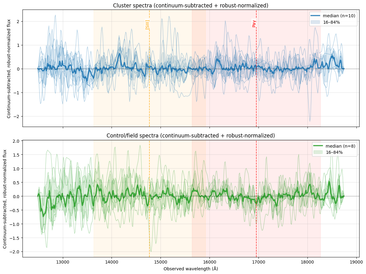
Figure 4 — Continuum-subtracted, normalized Euclid Q1 spectra for cluster (top) and control (bottom) samples. Thin lines show individual galaxy spectra; thick curves indicate the median, with shaded regions marking the 16–84 percentile range. Dashed vertical lines mark the expected observed wavelengths of prominent nebular emission lines at the cluster redshift, while shaded bands indicate the wavelength range allowed by the finite redshift slice of the sample. Spectra are not stacked in redshift; the figure is intended to highlight relative excess emission in physically motivated regions. Euclid Q1 spectra contain known instrumental artifacts that are addressed in DR1, so better results to be seen in the future.
8. NED Database Search
We search the NASA/IPAC Extragalactic Database (NED) for spectroscopically confirmed objects within 3 arcmin of both the cluster and control field centers, filtered to the cluster redshift slice. This provides an independent check of cluster membership using spectroscopic redshifts and lets us verify that the control field contains no known structures at the cluster redshift.
def search_ned_field(ra, dec, z_min, z_max, label, radius_arcmin=3, max_retries=3):
    """Search NED within radius_arcmin of (ra, dec), filter to z_min–z_max, and print a summary.

    Returns
    -------
    objects : astropy Table or None
        Rows in the redshift range, or None on failure.
    ned_ra_col, ned_dec_col : str or None
        Names of the RA and Dec columns in the returned table.
    ned_coord_unit : tuple or None
        Unit tuple suitable for SkyCoord construction.
    """
    ra_candidates  = ['RA(deg)', 'RA_deg', 'RA', 'RAJ2000']
    dec_candidates = ['DEC(deg)', 'DEC_deg', 'DEC', 'DEJ2000']

    def pick_col(table, candidates):
        for c in candidates:
            if c in table.colnames:
                return c
        return None

    center = SkyCoord(ra=ra, dec=dec, unit='deg')

    for attempt in range(max_retries):
        try:
            results = Ned.query_region(center, radius=radius_arcmin * u.arcmin)

            has_z = np.isfinite(np.asarray(results['Redshift'], float))
            objects_with_z = results[has_z]
            in_z_range = (objects_with_z['Redshift'] >= z_min) & (objects_with_z['Redshift'] <= z_max)
            objects = objects_with_z[in_z_range]

            print(f"{label}: {len(results)} total NED objects, {len(objects_with_z)} with redshift, "
                  f"{len(objects)} in z={z_min:.2f}–{z_max:.2f}")

            ned_ra_col  = pick_col(results, ra_candidates)
            ned_dec_col = pick_col(results, dec_candidates)
            if ned_ra_col is None or ned_dec_col is None:
                raise KeyError(f"Could not find RA/Dec columns. Available: {results.colnames}")

            ra_unit_str = str(getattr(results[ned_ra_col], 'unit', '')).lower()
            use_deg = 'deg' in ra_unit_str or 'deg' in ned_ra_col.lower()
            ned_coord_unit = ('deg', 'deg') if use_deg else (u.hourangle, u.deg)

            if len(objects) > 0:
                for obj in objects:
                    obj_coord = SkyCoord(ra=obj[ned_ra_col], dec=obj[ned_dec_col], unit=ned_coord_unit)
                    sep = center.separation(obj_coord).to(u.arcmin).value
                    print(f"  {obj['Object Name']} - {obj['Type']} - z={obj['Redshift']:.3f} - {sep:.1f}'")
                types = np.array([str(t) for t in objects['Type']], dtype=str)
                unique, counts = np.unique(types, return_counts=True)
                print("  Types:", dict(zip(unique, counts)))
            else:
                print("  No objects found in redshift range")

            return objects, ned_ra_col, ned_dec_col, ned_coord_unit

        except (Timeout, ConnectionError) as e:
            if attempt < max_retries - 1:
                time.sleep(5)
            else:
                print(f"{label}: NED search failed after {max_retries} attempts")
        except (RemoteServiceError, OSError, KeyError) as e:
            print(f"{label}: NED search error: {e}")
            break

    return None, None, None, None
z_min, z_max = cluster_z - 0.06, cluster_z + 0.06
cluster_objects, ned_ra_col, ned_dec_col, ned_coord_unit = search_ned_field(
cluster_ra, cluster_dec, z_min, z_max, label="Cluster field"
)Cluster field: NED search failed after 3 attempts
We repeat the search at the control field center to confirm that no previously catalogued structures fall within the comparison region.
control_objects, *_ = search_ned_field(
    control_ra, control_dec, z_min, z_max, label="Control field"
)
Control field: 855 total NED objects, 12 with redshift, 1 in z=0.49–0.61
WISEA J033406.21-280745.8 - G - z=0.544 - 0.9'
Types: {np.str_('G'): np.int64(1)}
We now overlay the NED-catalogued objects on the cluster and control field images to see how the spectroscopically confirmed sources (from NED) are spatially related to the photometric cluster members found by DBSCAN.
def overlay_ned_sources(
    cluster_objects, control_objects,
    ned_ra_col, ned_dec_col, ned_coord_unit,
    cluster_rgb, control_rgb,
    cluster_cutout_wcs, control_cutout_wcs,
    cluster_labels, cluster_galaxy_coords,
    control_labels, control_galaxy_coords,
):
    if cluster_objects is None or len(cluster_objects) == 0:
        print("No cluster NED objects to overlay.")
        return

    fig, (ax1, ax2) = plt.subplots(1, 2, figsize=(20, 8),
                                   subplot_kw={'projection': cluster_cutout_wcs})

    for ax, rgb, labels, coords, ned_objs, wcs, title in [
        (ax1, cluster_rgb, cluster_labels, cluster_galaxy_coords,
         cluster_objects, cluster_cutout_wcs, 'Cluster Field with NED Sources'),
        (ax2, control_rgb, control_labels, control_galaxy_coords,
         control_objects if control_objects is not None else [], control_cutout_wcs, 'Control Field'),
    ]:
        ax.imshow(rgb, origin='lower', alpha=0.3)

        unique_labels = set(labels)
        colors = plt.cm.Spectral(np.linspace(0, 1, len(unique_labels)))
        for k, col in zip(unique_labels, colors):
            if k == -1:
                continue  # noise points not shown
            mask = (labels == k)
            xy = coords[mask]
            if len(xy) > 0:
                ax.scatter(xy[:, 0], xy[:, 1], c='red', marker='o', s=20, alpha=0.8,
                           edgecolors='white', linewidth=0.5)

        for obj in ned_objs:
            ned_coord = SkyCoord(ra=obj[ned_ra_col], dec=obj[ned_dec_col], unit=ned_coord_unit)
            ned_pixel = wcs.world_to_pixel(ned_coord)
            if (0 <= ned_pixel[0] < rgb.shape[1] and 0 <= ned_pixel[1] < rgb.shape[0]):
                ax.scatter(ned_pixel[0], ned_pixel[1], facecolors='none', marker='o', s=100,
                           alpha=0.9, edgecolors='blue', linewidth=3)

        ax.set_title(title, fontsize=14, fontweight='bold')
        ax.set_xlabel('RA')
        ax.set_ylabel('Dec')

    handles = [
        plt.Line2D([0], [0], marker='o', color='none', linestyle='None',
                   markersize=8, markeredgecolor='blue', markeredgewidth=2),
        plt.Line2D([0], [0], marker='o', color='red', linestyle='None',
                   markersize=8, alpha=0.8),
    ]
    fig.legend(handles, ['NED Galaxy', 'Euclid Cluster Members'],
               loc='upper center', bbox_to_anchor=(0.5, 0.95), ncol=2, fontsize=10)

    plt.tight_layout()
    plt.show()
overlay_ned_sources(
cluster_objects, control_objects,
ned_ra_col, ned_dec_col, ned_coord_unit,
cluster_rgb, control_rgb,
cluster_cutout_wcs, control_cutout_wcs,
cluster_labels, cluster_galaxy_coords,
control_labels, control_galaxy_coords,
)No cluster NED objects to overlay.
Figure 5. Euclid DBSCAN cluster members and NED sources in cluster and control fields. Filled red circles are Euclid photometric cluster members identified by DBSCAN. Open blue circles are NED sources with spectroscopic redshifts in the cluster redshift slice; a blue circle overlapping a red dot indicates a source detected by both. The control field (right) contains no NED detections in the cluster redshift range, as expected for a blank field.
As a final validation, we cross-match the Euclid photometric cluster members against NED sources that have spectroscopic redshifts and compare their redshift estimates directly. Agreement between the Euclid photo-z values and the NED spectroscopic redshifts would confirm that our photometric selection is picking up real cluster members.
# Cross-match Euclid and NED sources for redshift comparison

# Get Euclid sources in cluster field
euclid_coords = SkyCoord(ra=cluster_members_cluster_field['ra'],
                        dec=cluster_members_cluster_field['dec'], unit='deg')
euclid_redshifts = cluster_members_cluster_field['phz_median'].values

# Get NED sources if available
if cluster_objects is not None and len(cluster_objects) > 0:
    if ned_ra_col and ned_dec_col:
        ned_coords = SkyCoord(ra=cluster_objects[ned_ra_col].data,
                             dec=cluster_objects[ned_dec_col].data, unit=ned_coord_unit)
        ned_redshifts = cluster_objects['Redshift'].data

        # Cross-match within 1 arcsec
        idx_ned, idx_euclid, d2d, d3d = search_around_sky(ned_coords, euclid_coords, 2*u.arcsec)

        if len(idx_ned) == 0:
            print("No cross-matches found between NED and Euclid sources within 2 arcsec.")
        else:
            print(f"Found {len(idx_ned)} matches between NED and Euclid sources within 2 arcsec")

            # Get matched redshifts
            ned_z_matched = ned_redshifts[idx_ned]
            euclid_z_matched = euclid_redshifts[idx_euclid]

            # Simple redshift comparison plot
            plt.figure(figsize=(8, 6))
            plt.scatter(euclid_z_matched, ned_z_matched, alpha=0.7, s=50)
            plt.plot([0, 1], [0, 1], 'r--', alpha=0.5, label='Perfect match')

            # Add cluster redshift reference lines
            plt.axvline(cluster_z, color='orange', linestyle=':', alpha=0.7, label=f'Cluster z={cluster_z:.3f}')
            plt.axhline(cluster_z, color='orange', linestyle=':', alpha=0.7)

            plt.xlabel('Euclid Redshift')
            plt.ylabel('NED Redshift')
            plt.title('Redshift Comparison: Euclid vs NED')
            plt.legend()
            plt.grid(True, alpha=0.3)

            # Calculate and display statistics
            z_diff = ned_z_matched - euclid_z_matched
            mean_diff = np.mean(z_diff)
            std_diff = np.std(z_diff)

            plt.text(0.05, 0.95, f'Mean difference: {mean_diff:.4f}\nStd deviation: {std_diff:.4f}',
                    transform=plt.gca().transAxes, verticalalignment='top',
                    bbox=dict(boxstyle='round', facecolor='white', alpha=0.8))

            plt.tight_layout()
            plt.xlim(z_min-0.1,z_max+0.1)
            plt.ylim(z_min-0.1,z_max+0.1)
            plt.show()
Figure 6. Euclid–NED redshift comparison for cross-matched galaxies within 2″. This figure only appears when at least one match is found.
Acknowledgements
About this notebook
Authors: Shoubaneh Hemmati, Jessica Krick, Brigitta Sipőcz
Updated: 2026-04-23
Contact: IRSA Helpdesk with questions or problems.
Runtime: As of the date above, this notebook takes about 2 minutes 40 seconds to run to completion on a machine with 64 GB RAM and 16 CPU (Fornax Large server). This runtime is dependent on archive servers which means runtime will vary for users.