Learning Goals
By the end of this tutorial, you will:
Understand the basic characteristics of Euclid Q1 photo-z catalog and how to match it with MER mosaics.
Understand what PHZ catalogs are available and how to view the columns in those catalogs.
How to query with ADQL in the PHZ catalog to find galaxies between a redshift of 1.4 and 1.6.
Pull and plot a spectrum of one of the galaxies in that catalog.
Cutout an image of the galaxy to view it close up.
Learn how to upload images and catalogs to Firefly to inspect individual sources in greater detail.
Introduction
Euclid launched in July 2023 as a European Space Agency (ESA) mission with involvement by NASA. The primary science goals of Euclid are to better understand the composition and evolution of the dark Universe. The Euclid mission is providing space-based imaging and spectroscopy as well as supporting ground-based imaging to achieve these primary goals. These data will be archived by multiple global repositories, including IRSA, where they will support transformational work in many areas of astrophysics.
Euclid Quick Release 1 (Q1) consists of consists of ~30 TB of imaging, spectroscopy, and catalogs covering four non-contiguous fields: Euclid Deep Field North (22.9 sq deg), Euclid Deep Field Fornax (12.1 sq deg), Euclid Deep Field South (28.1 sq deg), and LDN1641.
Among the data products included in the Q1 release are multiple catalogs created by the PHZ Processing Function. This notebook provides an introduction to the main PHZ catalog, which contains 61 columns describing the photometric redshift probability distribution, fluxes, and classification for each source. If you have questions about this notebook, please contact the IRSA helpdesk.
Imports
# Uncomment the next line to install dependencies if needed.
# !pip install matplotlib 'astropy>=5.3' 'astroquery>=0.4.11' fsspec firefly_client
import os
import re
import io
import urllib
import numpy as np
import matplotlib.pyplot as plt
from astropy.coordinates import SkyCoord
from astropy.io import fits
from astropy.nddata import Cutout2D
from astropy.table import QTable
from astropy import units as u
from astropy.utils.data import conf, download_file
from astropy.visualization import ImageNormalize, PercentileInterval, AsinhStretch, LogStretch, quantity_support
from astropy.wcs import WCS
from firefly_client import FireflyClient
from astroquery.ipac.irsa import Irsa
# The Euclid spectrum files are large and the time it takes to read
# them can exceed astropy's default timeout limit. Increase it.
conf.remote_timeout = 1201. Find the MER Tile ID that corresponds to a given RA and Dec
In this case, choose random coordinates to show a different MER mosaic image. Search a radius around these coordinates.
ra = 268
dec = 66
search_radius= 10 * u.arcsec

coord = SkyCoord(ra, dec, unit='deg', frame='icrs')
Use IRSA to search for all Euclid data on this target
This searches specifically in the euclid_DpdMerBksMosaic “collection” which is the MER images and catalogs.
image_table = Irsa.query_sia(pos=(coord, search_radius), collection='euclid_DpdMerBksMosaic', facility='Euclid')Note that there are various image types are returned as well, we filter out the science images from these:
science_images = image_table[image_table['dataproduct_subtype'] == 'science']
science_imagesChoose the VIS image and pull the filename and tileID
filename = science_images[science_images['energy_bandpassname'] == 'VIS']['access_url'][0]
tileID = science_images[science_images['energy_bandpassname'] == 'VIS']['obs_id'][0][:9]

print(f'The MER tile ID for this object is : {tileID}')
The MER tile ID for this object is : 102159190
2. Download PHZ catalog from IRSA
Use IRSA’s TAP to search catalogs and metadata tables associated with Euclid:
Irsa.list_catalogs(filter='euclid', include_metadata_tables=True){'euclid.tileid_association_q1': 'Euclid Q1 TILEID to Observation ID Association Table',
'euclid.objectid_spectrafile_association_q1': 'Euclid Q1 Object ID to Spectral File Association Table',
'euclid.observation_euclid_q1': 'Euclid Q1 CAOM Observation Table',
'euclid.plane_euclid_q1': 'Euclid Q1 CAOM Plane Table',
'euclid.artifact_euclid_q1': 'Euclid Q1 CAOM Artifact Table',
'euclid_q1_mer_catalogue': 'Euclid Q1 MER Catalog',
'euclid_q1_mer_morphology': 'Euclid Q1 MER Morphology',
'euclid_q1_mer_cutouts': 'Euclid Q1 MER Cutouts',
'euclid_q1_phz_photo_z': 'Euclid Q1 PHZ Photo-z Catalog',
'euclid_q1_phz_star_sed': 'Euclid Q1 PHZ Star SED Catalog',
'euclid_q1_phz_galaxy_sed': 'Euclid Q1 PHZ Galaxy SED Catalog',
'euclid_q1_phz_classification': 'Euclid Q1 PHZ Classification Catalog',
'euclid_q1_phz_qso_physical_parameters': 'Euclid Q1 PHZ QSO Physical Parameters Catalog',
'euclid_q1_phz_nir_physical_parameters': 'Euclid Q1 PHZ NIR Physical Parameters Catalog',
'euclid_q1_phz_star_template': 'Euclid Q1 PHZ Star Template Catalog',
'euclid_q1_spectro_zcatalog_spe_quality': 'Euclid Q1 SPE Redshift Catalog - Quality',
'euclid_q1_spectro_zcatalog_spe_classification': 'Euclid Q1 SPE Redshift Catalog - Classification',
'euclid_q1_spectro_zcatalog_spe_galaxy_candidates': 'Euclid Q1 SPE Redshift Catalog - Galaxy Candidates',
'euclid_q1_spectro_zcatalog_spe_star_candidates': 'Euclid Q1 SPE Redshift Catalog - Star Candidates',
'euclid_q1_spectro_zcatalog_spe_qso_candidates': 'Euclid Q1 SPE Redshift Catalog - QSO Candidates',
'euclid_q1_spe_lines_line_features': 'Euclid Q1 SPE Lines Catalog - Spectral Lines',
'euclid_q1_spe_lines_continuum_features': 'Euclid Q1 SPE Lines Catalog - Continuum Features',
'euclid_q1_spe_lines_atomic_indices': 'Euclid Q1 SPE Lines Catalog - Atomic Indices',
'euclid_q1_spe_lines_molecular_indices': 'Euclid Q1 SPE Lines Catalog - Molecular Indices',
'euclid_q1_spectro_model_catalog_spe_lines_catalog': 'Euclid Q1 SPE Models Catalog - Lines',
'euclid_q1_spectro_model_catalog_spe_star_models': 'Euclid Q1 SPE Star Models Catalog'}table_mer = 'euclid_q1_mer_catalogue'
table_phz = 'euclid_q1_phz_photo_z'
table_1dspectra = 'euclid.objectid_spectrafile_association_q1'Learn some information about the photo-z catalog:
How many columns are there?
List the column names
columns_info = Irsa.list_columns(catalog=table_phz)
print(len(columns_info))
67
# Full list of columns and their description
columns_info
{'fluxerr_g_ext_lsst_unif': '',
'fluxerr_r_ext_lsst_unif': '',
'fluxerr_i_ext_lsst_unif': '',
'fluxerr_z_ext_lsst_unif': '',
'fluxerr_u_ext_megacam_unif': '',
'fluxerr_g_ext_hsc_unif': '',
'fluxerr_r_ext_megacam_unif': '',
'fluxerr_i_ext_panstarrs_unif': '',
'fluxerr_z_ext_hsc_unif': '',
'fluxerr_vis_unif': '',
'fluxerr_y_unif': '',
'fluxerr_j_unif': '',
'fluxerr_h_unif': '',
'photometric_system': 'Encode the Photometric band configuration (indicating also the number of missing columns)',
'phz_classification': 'Classification flag: 1 if the source is accepted as star, 2 if it is accepted as a galaxy, 4 if it is accepted as a QSO, 8 if the source is acce..."',
'phz_flags': 'An integer containing the flags of the PHZ processing. Meaning: 0 => OK, 1 => NNPZ flag: no close neighbor, 10 not VIS detected, 11 missing band, 12 t...',
'phz_weight': 'Probability to be a usable source at VIS MAG=23.5',
'best_chi2': 'Chi2 of the best fit model or the closest neighbor',
'phz_70_int1': 'The smallest PHZ PDF interval containing 70% of the probability - lower value',
'phz_70_int2': 'The smallest PHZ PDF interval containing 70% of the probability - upper value',
'phz_90_int1': 'The smallest PHZ PDF interval containing 90% of the probability - lower value',
'phz_90_int2': 'The smallest PHZ PDF interval containing 90% of the probability - upper value',
'phz_95_int1': 'The smallest PHZ PDF interval containing 95% of the probability - upper value',
'phz_95_int2': '',
'ie_cuts_weights1': 'Vector of probability to be a usable source for VIS MAG cut 20.25',
'ie_cuts_weights2': 'Vector of probability to be a usable source for VIS MAG cut 21.25',
'ie_cuts_weights3': 'Vector of probability to be a usable source for VIS MAG cut 22.25',
'ie_cuts_weights4': 'Vector of probability to be a usable source for VIS MAG cut 24.5',
'cntr': 'entry counter (key) number (unique within table)',
'object_id': 'Unique ID of the object in the survey, as set by MER',
'phz_median': 'The median of the PHZ PDF',
'phz_mode_1': 'The first mode of the PHZ PDF',
'phz_mode_1_area': 'The total area of the first mode',
'phz_mode_2': 'The second mode of the PHZ PDF',
'phz_mode_2_area': 'The total area of the second mode',
'bias_id': 'The identifier to be used for retrieving the bias correction shift from the bias correction map',
'tom_bin_id': 'The identifier of the tomographic bin the source belongs to (Equipopulated-bins)',
'alt_tom_bin_id': 'The identifier of the alternate tomographic bin the source belongs to (Equidistant-bins)',
'pos_tom_bin_id': 'The identifier of the photometric clustering tomographic bin the source belongs to (Equipopulated-bins)',
'flag_som_tomobin': 'Flag telling if the source belong to a combination of SOM cell and Tom. bin which can be calibrated (=1) or not (=0).',
'flag_som_alt_tomobin': 'Flag telling if the source belong to a combination of SOM cell and Alt Tom. bin which can be calibrated (=1) or not (=0).',
'flag_som_pos_tomobin': 'Flag telling if the source belong to a combination of SOM cell and POS Tom. bin which can be calibrated (=1) or not (=0).',
'flux_u_ext_decam_unif': 'Unified flux recomputed after correction from galactic extinction and filter shifts',
'flux_g_ext_decam_unif': '',
'flux_r_ext_decam_unif': '',
'flux_i_ext_decam_unif': '',
'flux_z_ext_decam_unif': '',
'flux_u_ext_lsst_unif': '',
'flux_g_ext_lsst_unif': '',
'flux_r_ext_lsst_unif': '',
'flux_i_ext_lsst_unif': '',
'flux_z_ext_lsst_unif': '',
'flux_u_ext_megacam_unif': '',
'flux_g_ext_hsc_unif': '',
'flux_r_ext_megacam_unif': '',
'flux_i_ext_panstarrs_unif': '',
'flux_z_ext_hsc_unif': '',
'flux_vis_unif': '',
'flux_y_unif': '',
'flux_j_unif': '',
'flux_h_unif': '',
'fluxerr_u_ext_decam_unif': '',
'fluxerr_g_ext_decam_unif': '',
'fluxerr_r_ext_decam_unif': '',
'fluxerr_i_ext_decam_unif': '',
'fluxerr_z_ext_decam_unif': '',
'fluxerr_u_ext_lsst_unif': ''}Find some galaxies between 1.4 and 1.6 at a selected RA and Dec
We specify the following conditions on our search:
We select just the galaxies where the flux is greater than zero, to ensure the appear in all four of the Euclid MER images.
Select only objects in a circle (search radius selected below) around our selected RA and Dec
phz_classification = 2means we select only galaxiesUsing the
phz_90_int1andphz_90_int2, we select just the galaxies where the error on the photometric redshift is less than 20%Select just the galaxies between a median redshift of 1.4 and 1.6
We search just a 5 arcminute box around an RA and Dec
Search based on tileID:
######################## User defined section ############################
# Set the image cutout size
im_cutout= 5 * u.arcmin

# Set the center of the cutout
ra_cutout = 267.8
dec_cutout =  66

coords_cutout = SkyCoord(ra_cutout, dec_cutout, unit='deg', frame='icrs')
size_cutout = im_cutout.to(u.deg).value
adql = ("SELECT DISTINCT mer.object_id, mer.ra, mer.dec, "
"phz.flux_vis_unif, phz.flux_y_unif, phz.flux_j_unif, phz.flux_h_unif, "
"phz.phz_classification, phz.phz_median, phz.phz_90_int1, phz.phz_90_int2 "
f"FROM {table_mer} AS mer "
f"JOIN {table_phz} as phz "
"ON mer.object_id = phz.object_id "
"WHERE 1 = CONTAINS(POINT('ICRS', mer.ra, mer.dec), "
f"BOX('ICRS', {ra_cutout}, {dec_cutout}, {size_cutout/np.cos(coords_cutout.dec)}, {size_cutout})) "
"AND phz.flux_vis_unif> 0 "
"AND phz.flux_y_unif > 0 "
"AND phz.flux_j_unif > 0 "
"AND phz.flux_h_unif > 0 "
"AND phz.phz_classification = 2 "
"AND ((phz.phz_90_int2 - phz.phz_90_int1) / (1 + phz.phz_median)) < 0.20 "
"AND phz.phz_median BETWEEN 1.4 AND 1.6")
# Use TAP with this ADQL string
result_galaxies = Irsa.query_tap(adql).to_table()
result_galaxies[:5]3. Read in a cutout of the MER image from IRSA directly
Due to the large field of view of the MER mosaic, let’s cut out a smaller section (5’x5’) of the MER mosaic to inspect the image.
# Use fsspec to interact with the fits file without downloading the full file
hdu = fits.open(filename, use_fsspec=True)

# Store the header
header = hdu[0].header

# Read in the cutout of the image that you want
cutout_image = Cutout2D(hdu[0].section, position=coords_cutout, size=im_cutout, wcs=WCS(header))cutout_image.data.shape(3000, 3000)norm = ImageNormalize(cutout_image.data, interval=PercentileInterval(99.9), stretch=AsinhStretch())
_ = plt.imshow(cutout_image.data, cmap='gray', origin='lower', norm=norm)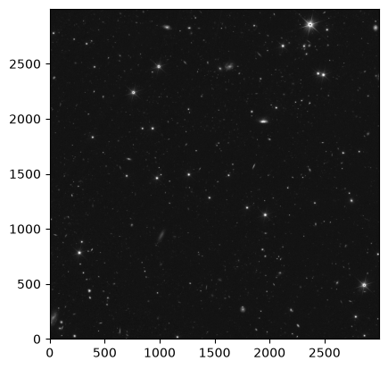
4. Overplot the catalog on the MER mosaic image
ax = plt.subplot(projection=cutout_image.wcs)

ax.imshow(cutout_image.data, cmap='gray', origin='lower',
          norm=ImageNormalize(cutout_image.data, interval=PercentileInterval(99.9), stretch=LogStretch()))
plt.scatter(result_galaxies['ra'], result_galaxies['dec'], s=36, facecolors='none', edgecolors='red',
            transform=ax.get_transform('world'))

_ = plt.title('Galaxies between z = 1.4 and 1.6')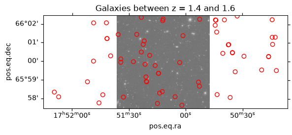
5. Pull spectra for one of the brightest sources by object ID
result_galaxies.sort(keys='flux_h_unif', reverse=True)result_galaxies[:3]Let’s pick one of these galaxies. Note that the table has been sorted above, we can use the same index here and below to access the data for this particular galaxy.
index = 2

obj_id = result_galaxies['object_id'][index]
redshift = result_galaxies['phz_median'][index]
We will use TAP and an ASQL query to find the spectral data for this particular galaxy.
adql_object = f"SELECT * FROM {table_1dspectra} WHERE objectid = {obj_id}"

# Pull the data on this particular galaxy
result_spectra = Irsa.query_tap(adql_object).to_table()
result_spectraPull out the file name from the result_spectra table:
spectrum_path = f"https://irsa.ipac.caltech.edu/{result_spectra['path'][0]}"
spectrum_path'https://irsa.ipac.caltech.edu/api/spectrumdm/convert/euclid/q1/SIR/102159190/EUC_SIR_W-COMBSPEC_102159190_2024-11-05T16:17:13.710030Z.fits?dataset_id=euclid_combspec&hdu=1474'spectrum = QTable.read(spectrum_path)WARNING: UnitsWarning: The unit 'Angstrom' has been deprecated in the VOUnit standard. Suggested: 0.1nm. [astropy.units.format.base]
WARNING: UnitsWarning: The unit 'erg' has been deprecated in the VOUnit standard. Suggested: cm**2.g.s**-2. [astropy.units.format.base]
WARNING: UnitsWarning: The unit 'Angstrom' has been deprecated in the VOUnit standard. Suggested: 0.1nm. [astropy.units.format.base]
WARNING: UnitsWarning: The unit 'erg' has been deprecated in the VOUnit standard. Suggested: cm**2.g.s**-2. [astropy.units.format.base]
WARNING: UnitsWarning: The unit 'Angstrom' has been deprecated in the VOUnit standard. Suggested: 0.1nm. [astropy.units.format.base]
WARNING: UnitsWarning: The unit 'erg' has been deprecated in the VOUnit standard. Suggested: cm**2.g.s**-2. [astropy.units.format.base]
WARNING: UnitsWarning: The unit 'Angstrom' has been deprecated in the VOUnit standard. Suggested: 0.1nm. [astropy.units.format.base]
Now the data are read in, plot the spectrum
quantity_support()<astropy.visualization.units.quantity_support.<locals>.MplQuantityConverterFormatted at 0x7f0f7076aab0>plt.plot(spectrum['WAVELENGTH'].to(u.micron), spectrum['SIGNAL'])
plt.xlim(1.25, 1.85)
plt.ylim(-0.5, 0.5)
_ = plt.title(f"Object {obj_id} with phz_median={redshift}")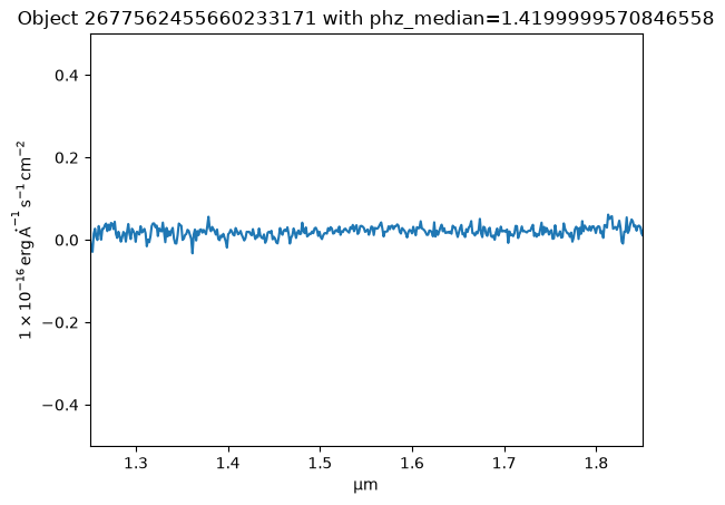
Let’s cut out a very small patch of the MER image to see what this galaxy looks like. Remember that we sorted the table above, so can reuse the same index to pick up the coordinates for the galaxy. Otherwise we could filter on the object ID.
result_galaxies[index]# Set the image cutout size for the selected galaxy
size_galaxy_cutout = 2.0 * u.arcsecUse the ra and dec columns for the galaxy to create a SkyCoord.
coords_galaxy = SkyCoord(result_galaxies['ra'][index], result_galaxies['dec'][index], unit='deg')coords_galaxy<SkyCoord (ICRS): (ra, dec) in deg
(267.75624552, 66.02331715)>We haven’t closed the image file above, so use Cutout2D again to cut out a section around the galaxy.
cutout_galaxy = Cutout2D(hdu[0].section, position=coords_galaxy, size=size_galaxy_cutout, wcs=WCS(header))Plot to show the cutout on the galaxy
ax = plt.subplot(projection=cutout_galaxy.wcs)

ax.imshow(cutout_galaxy.data, cmap='gray', origin='lower',
          norm=ImageNormalize(cutout_galaxy.data, interval=PercentileInterval(99.9), stretch=AsinhStretch()))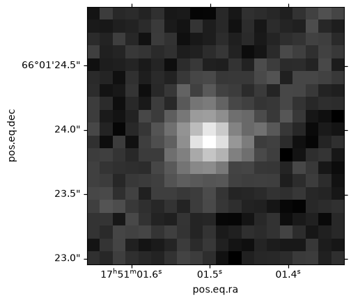
6. Load the image in Firefly for interactive exploration
First we intialize the Firefly client as explained here so that we can send our data to Firefly for visualization.
fc = FireflyClient.make_client('https://irsa.ipac.caltech.edu/irsaviewer')Vizualize the FITS image with Firefly
After initializing the client, we can directly use the FITS image file URL to visualise it in Firefy.
Note this can take a while to upload the full MER image.
fc.show_fits_image(filename){'success': True}Display the table as an overlay on the FITS image
Since our galaxies table is in memory, we write it to an IO stream (file-like object) for visualizing it in Firefly. Besides displaying the table, Firefly will also overlay the positions of the galaxies on the FITS image we visualized earlier. You can click on a table row to inspect the particular galaxy in the image, or click on an overlay marker to inspect the particular galaxy in the table.
tbl_stream = io.BytesIO()
result_galaxies.write(tbl_stream, format='votable')

fc.show_table(tbl_stream)
{'success': True}About this Notebook
Updated: 2026-04-29
Contact: the IRSA Helpdesk with questions or reporting problems.