This tutorial explores Euclid photometry measurements. It assumes you are familiar with the first tutorial in this series, which covers the Euclid Q1 Merged Objects HATS Catalog content, format, and basic access.
Learning Goals
By the end of this tutorial, you will be able to:
Understand the different Euclid Q1 flux measurements and their intended use cases.
Load aperture and template-fit magnitudes for Euclid I, Y, J, and H bands from the Euclid Q1 Merged Objects HATS Catalog.
Visualize and understand the template-fit magnitude distributions as a function of object classification.
Compare aperture and template-fit magnitudes to understand their differences.
1. Introduction
The Euclid Q1 data release contains photometry from Euclid as well as from external surveys. There are several flux measurements per band. The measurements are described in Euclid Collaboration: Romelli et al., 2025 (hereafter, Romelli), especially sections 6 and 8.
In this tutorial, we will look at aperture and template-fit photometry measurements in the four Euclid bands: I (from the VIS instrument), Y, J, and H (from the NISP instrument). Aperture fluxes are generally more accurate for point-like sources, especially bright stars in the NIR bands, likely due to better handling of PSF-related effects. Template-fit fluxes are expected to be more accurate for extended sources because the templates do a better job of excluding contamination from nearby sources. Additional photometry measurements that we won’t cover here include: Sérsic-fit fluxes (computed for parametric morphology), PSF-fit fluxes (VIS only), and class-corrected fluxes that were corrected based on the PHZ (photometric) classifications.
The best-estimate flux in the detection band is given by the column mer_flux_detection_total.
This can also be used to color-correct flux measurements in non-detection bands, as we will demonstrate.
The object detection process is described in Romelli.
The MER Photometry Cookbook describes the color corrections and how to convert from flux to magnitude.
In this tutorial, we will restrict to objects detected in VIS (I band) because it simplifies the calculations.
2. Imports and Paths
# # Uncomment the next line to install dependencies if needed.
# %pip install hpgeom matplotlib pandas pyarrow
import hpgeom # Find HEALPix indexes from RA and Dec
import matplotlib.pyplot as plt # Create figures
import pyarrow.compute as pc # Filter dataset
import pyarrow.dataset # Load the dataset
import pyarrow.fs # Simple S3 filesystem pointer
import pyarrow.parquet # Load the schema
# Increase font size in figures.
plt.rcParams.update({"font.size": 14})# AWS S3 paths.
s3_bucket = "nasa-irsa-euclid-q1"
dataset_prefix = "contributed/q1/merged_objects/hats/euclid_q1_merged_objects-hats/dataset"
dataset_path = f"{s3_bucket}/{dataset_prefix}"
# S3 pointer. Use `anonymous=True` to access without credentials.
s3 = pyarrow.fs.S3FileSystem(anonymous=True)3. Load Template-fit and Aperture Magnitudes
The following columns will be important. Descriptions come from Romelli.
# Whether the source was detected in VIS mosaic (1) or only in NIR-stack mosaic (0).
VIS_DET = "mer_vis_det"

# Best estimate of the total flux in the detection band.
# From aperture photometry within a Kron radius.
# Detection band is VIS if `VIS_DET == 1`. Otherwise, this is a
# non-physical NIR-stack flux and there was no VIS detection (aka, NIR-only).
# We will only deal with VIS-detected objects in this notebook.
FLUX_DET_TOTAL = "mer_flux_detection_total"

# Peak surface brightness minus the magnitude used for `mer_point_like_prob`.
# This is a measure of compactness.
MUMAX_MINUS_MAG = "mer_mumax_minus_mag"

# Whether the detection has a >50% probability of being spurious (1=Yes, 0=No).
SPURIOUS_FLAG = "mer_spurious_flag"

# PHZ classification: 1=Star, 2=Galaxy, 4=QSO.
# Combinations (3, 5, 6, and 7) indicate multiple probability thresholds were exceeded.
PHZ_CLASS = "phz_phz_classification"
We’ll convert the catalog fluxes to magnitudes following the MER Photometry Cookbook.
PyArrow can do the conversion during the read operation and return only the magnitudes.
To do this, we’ll use the following function to define the magnitudes as pyarrow.compute (pc) functions, which are described at Compute Functions.
def flux_to_magnitude(flux_col_name: str) -> pc.Expression:
    """Convert catalog fluxes to magnitudes following the MER Photometry Cookbook.

    Parameters
    ----------
    flux_col_name : str
        The name of the flux column to convert to magnitude.

    Returns
    -------
    pyarrow.compute.Expression
        An expression for the magnitude. It can be used in the `filter` and `columns`
        keyword arguments when loading data from a PyArrow dataset.
    """
    # We expect to be dealing with VIS_DET == 1 objects, so FLUX_DET_TOTAL == VIS flux.
    vis_flux = pc.field(FLUX_DET_TOTAL)
    band_flux = pc.field(flux_col_name)

    if flux_col_name == FLUX_DET_TOTAL:
        # Best-estimate flux in VIS is FLUX_DET_TOTAL.
        best_flux = vis_flux
    elif flux_col_name.endswith("_templfit"):
        # Best-estimate template-fit flux is the band flux scaled by a color correction.
        band = flux_col_name.split("_")[-2]  # y, j, or h
        color_scale = pc.divide(vis_flux, pc.field(f"mer_flux_vis_to_{band}_templfit"))
        best_flux = pc.multiply(band_flux, color_scale)
    elif flux_col_name.endswith("aper"):
        # Best-estimate aperture flux is the band flux scaled by a color correction.
        nfwhm = flux_col_name.split("_")[-2]  # e.g., 2fwhm
        color_scale = pc.divide(vis_flux, pc.field(f"mer_flux_vis_{nfwhm}_aper"))
        best_flux = pc.multiply(band_flux, color_scale)

    # magnitude = -2.5 * log10(flux) + 23.9.
    scale = pc.scalar(-2.5)
    log10_flux = pc.log10(best_flux)
    zeropoint = pc.scalar(23.9)
    mag_expression = pc.add(pc.multiply(scale, log10_flux), zeropoint)
    return mag_expression
Define the columns we want to load.
This needs to be a dictionary (rather than a simple list of column names) because we’re asking PyArrow to compute the magnitudes dynamically from the catalog fluxes.
The dictionary keys will be the column names in the resultant table.
The values must be pyarrow.compute expressions (described above).
I_MAG = "I (mag)"
columns = {
    PHZ_CLASS: pc.field(PHZ_CLASS),
    I_MAG: flux_to_magnitude(FLUX_DET_TOTAL),
    "Y aperture (mag)": flux_to_magnitude("mer_flux_y_2fwhm_aper"),
    "J aperture (mag)": flux_to_magnitude("mer_flux_j_2fwhm_aper"),
    "H aperture (mag)": flux_to_magnitude("mer_flux_h_2fwhm_aper"),
    "Y templfit (mag)": flux_to_magnitude("mer_flux_y_templfit"),
    "J templfit (mag)": flux_to_magnitude("mer_flux_j_templfit"),
    "H templfit (mag)": flux_to_magnitude("mer_flux_h_templfit"),
    MUMAX_MINUS_MAG: pc.field(MUMAX_MINUS_MAG),
}
# Let's see what one of these looks like.
columns["Y aperture (mag)"]
<pyarrow.compute.Expression add(multiply(-2.5, log10(multiply(mer_flux_y_2fwhm_aper, divide(mer_flux_detection_total, mer_flux_vis_2fwhm_aper)))), 23.9)>We’ll restrict to the Euclid Deep Field - Fornax (EDF-F) to reduce the amount of data loaded. Compute the HEALPix order 9 pixel indexes, following the introductory tutorial.
ra, dec, radius = 52.932, -28.088, 3  # 10 sq deg
edff_k9_pixels = hpgeom.query_circle(hpgeom.order_to_nside(9), ra, dec, radius, inclusive=True)
Construct the row filter.
row_filter = (
    # Stars, Galaxies, QSOs, and mixed classes.
    pc.field(PHZ_CLASS).isin([1, 2, 3, 4, 5, 6, 7])
    # Basic quality cut.
    & (pc.field(SPURIOUS_FLAG) == 0)
    # VIS-detected objects. (If you want to include NIR-only objects, alter flux_to_magnitude()
    # following MER Photometry Cookbook and also comment out the next line.)
    & (pc.field(VIS_DET) == 1)
    # EDF-F region. (Comment out the next line to do an all-sky search.)
    & pc.field("_healpix_9").isin(edff_k9_pixels)
)
Load the data.
# Load the catalog as a PyArrow dataset. Include partitioning="hive"
# so PyArrow understands the file naming scheme and can navigate the partitions.
schema = pyarrow.parquet.read_schema(f"{dataset_path}/_common_metadata", filesystem=s3)
dataset = pyarrow.dataset.dataset(dataset_path, partitioning="hive", filesystem=s3, schema=schema)

mags_df = dataset.to_table(columns=columns, filter=row_filter).to_pandas()
mags_df4. Magnitude Distributions of Galaxies, Stars, and QSOs
Let’s visualize the template-fit magnitude distributions as a function of PHZ classification.
Since the template-fit photometry is recommended for extended objects, we’ll separate the point-like objects.
Euclid Collaboration: Tucci et al., 2025 defines point-like objects as having MUMAX_MINUS_MAG < -2.5.
# Galaxy + any. Star + galaxy. QSO + galaxy.
classes = {"Galaxy": (2, 3, 6, 7), "Star": (1, 3), "QSO": (4, 6)}
class_colors = ["tab:green", "tab:blue", "tab:orange"]

bands = [I_MAG, "Y templfit (mag)", "J templfit (mag)", "H templfit (mag)"]
mag_limits = (14, 28)  # Excluding all magnitudes outside this range.
hist_kwargs = dict(bins=20, range=mag_limits, histtype="step")

fig, axes = plt.subplots(3, 4, figsize=(18, 12), sharey="row", sharex=True)
for (class_name, class_ids), class_color in zip(classes.items(), class_colors):
    hist_kwargs["color"] = class_color

    # Get the objects that are in this class only.
    class_df = mags_df.loc[mags_df[PHZ_CLASS] == class_ids[0]]
    # Plot histograms for each band. Galaxies on top row, then stars, then QSOs.
    axs = axes[0] if class_name == "Galaxy" else (axes[1] if class_name == "Star" else axes[2])
    for ax, band in zip(axs, bands):
        ax.hist(class_df[band], label=class_name, **hist_kwargs)

    # Get the objects that were accepted as multiple classes.
    class_df = mags_df.loc[mags_df[PHZ_CLASS].isin(class_ids)]
    label = "+Galaxy" if class_name != "Galaxy" else "+any"
    # Of those objects, restrict to the ones that are point-like.
    classpt_df = class_df.loc[class_df[MUMAX_MINUS_MAG] < -2.5]
    pt_label = f"{label} (point-like)"
    # Plot histograms for both sets of objects.
    for ax, band in zip(axs, bands):
        ax.hist(class_df[band], label=label, linestyle=":", **hist_kwargs)
        ax.hist(classpt_df[band], linestyle="-.", label=pt_label, **hist_kwargs)

# Add axis labels, etc.
for ax, loc in zip(axes[:, 0], [2, 3, 2]):
    ax.legend(loc=loc)
    ax.set_ylabel("Counts")
for axs, band in zip(axes.transpose(), bands):
    axs[0].set_title(band.split()[0])
    axs[-1].set_xlabel(band)
fig.suptitle("Magnitude Distributions by Object Type")
plt.tight_layout()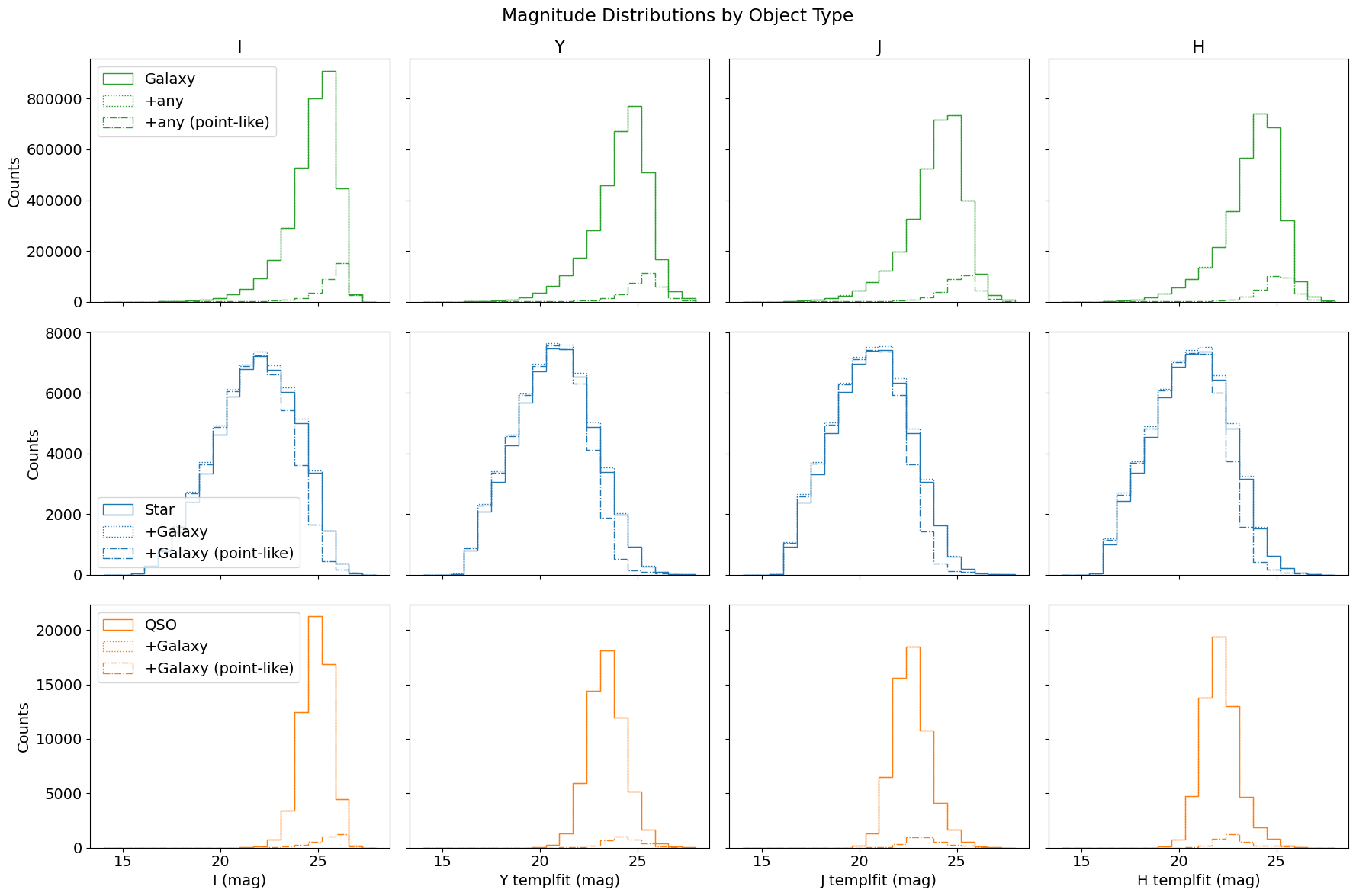
The Euclid instruments are tuned to detect galaxies for cosmology studies, so it’s no surprise that there are many more galaxies than other object types.
The green lines (top row) show the magnitude distributions of objects classified as galaxy only (solid) and those classified as galaxy plus possibly other types (dot and dash-dot). The dash-dot line highlights the population of point-like “galaxies”, which are likely misclassified stars or QSOs and mostly appear at faint magnitudes.
The star distributions (middle row, blue) are broader and peak at brighter magnitudes than the galaxy distributions, as expected. Adding objects classified as both star and galaxy (dotted line) adds significant numbers, especially near the peak and toward the faint end where confusion is more likely. Restricting these to point-like objects (dash-dot line) shows that many bright objects surpassing both probability thresholds are likely to be stars, not galaxies. However, this doesn’t hold at the faint end where even some star-only classified objects fail the point-like cut.
The bottom row (orange) is the same as the middle row but for QSOs instead of stars. There are very few point-like QSOs, reminding us that most QSO classifications in Q1 should be treated with skepticism (as discussed in the Classifications tutorial). By default, this figure only includes objects in the EDF-F region. High-confidence QSOs are more concentrated in the EDF-N region where advantageous external photometry (particularly u-band from UNIONS) was available.
5. Template-fit vs. Aperture Magnitudes
Now let’s compare template-fit and aperture magnitudes by plotting their differences. This comparison reveals systematic offsets that depend on factors including morphology (extended vs. point-like) and brightness.
This figure is inspired by Romelli Fig. 6 (top panel).
# Only consider objects within these mag and mag difference limits.
mag_limits, mag_diff_limits = (16, 24), (-1, 1)
mag_limited_df = mags_df.loc[(mags_df[I_MAG] > mag_limits[0]) & (mags_df[I_MAG] < mag_limits[1])]

bands = [
    ("Y templfit (mag)", "Y aperture (mag)"),
    ("J templfit (mag)", "J aperture (mag)"),
    ("H templfit (mag)", "H aperture (mag)"),
]
hexbin_kwargs = dict(
    cmap="YlGnBu", bins="log", extent=(*mag_limits, *mag_diff_limits), gridsize=25
)
annotate_kwargs = dict(
    xycoords="axes fraction", ha="left", fontweight="bold", bbox=dict(facecolor="white", alpha=0.8)
)

# Plot
fig, axes = plt.subplots(2, 3, figsize=(18, 9), sharey=True, sharex=True)
for axs, (ref_band, aper_band) in zip(axes.transpose(), bands):
    # Extended objects, top row.
    ax = axs[0]
    extended = mags_df.loc[mags_df[MUMAX_MINUS_MAG] >= -2.5, [I_MAG, ref_band, aper_band]]
    extended["mag_diff"] = extended[ref_band] - extended[aper_band]
    extended = extended.dropna(subset="mag_diff")
    cb = ax.hexbin(extended[I_MAG], extended["mag_diff"], **hexbin_kwargs)
    plt.colorbar(cb)
    ax.set_ylabel(f"{ref_band} - {aper_band}")
    # Annotate top (bottom) with the fraction of objects having a magnitude difference greater (less) than 0.
    frac_tmpl_greater = len(extended.loc[extended["mag_diff"] > 0]) / len(extended)
    ax.annotate(f"{frac_tmpl_greater:.3f}", xy=(0.01, 0.99), va="top", **annotate_kwargs)
    frac_tmpl_less = len(extended.loc[extended["mag_diff"] < 0]) / len(extended)
    ax.annotate(f"{frac_tmpl_less:.3f}", xy=(0.01, 0.01), va="bottom", **annotate_kwargs)

    # Point-like objects, bottom row.
    ax = axs[1]
    pointlike = mags_df.loc[mags_df[MUMAX_MINUS_MAG] < -2.5, [I_MAG, ref_band, aper_band]]
    pointlike["mag_diff"] = pointlike[ref_band] - pointlike[aper_band]
    pointlike = pointlike.dropna(subset="mag_diff")
    cb = ax.hexbin(pointlike[I_MAG], pointlike["mag_diff"], **hexbin_kwargs)
    plt.colorbar(cb)
    ax.set_ylabel(f"{ref_band} - {aper_band}")
    # Annotate top (bottom) with the fraction of objects having a magnitude difference greater (less) than 0.
    frac_tmpl_greater = len(pointlike.loc[pointlike["mag_diff"] > 0]) / len(pointlike)
    ax.annotate(f"{frac_tmpl_greater:.3f}", xy=(0.01, 0.99), va="top", **annotate_kwargs)
    frac_tmpl_less = len(pointlike.loc[pointlike["mag_diff"] < 0]) / len(pointlike)
    ax.annotate(f"{frac_tmpl_less:.3f}", xy=(0.01, 0.01), va="bottom", **annotate_kwargs)

# Add axis labels, etc.
for i, ax in enumerate(axes.flatten()):
    ax.axhline(0, color="gray", linewidth=1)
    if i == 1:
        ax.set_title("Extended objects")
    if i == 4:
        ax.set_title("Point-like objects")
    if i > 2:
        ax.set_xlabel(I_MAG)
fig.suptitle("Magnitude Offsets (Template fit - Aperture)")
plt.tight_layout()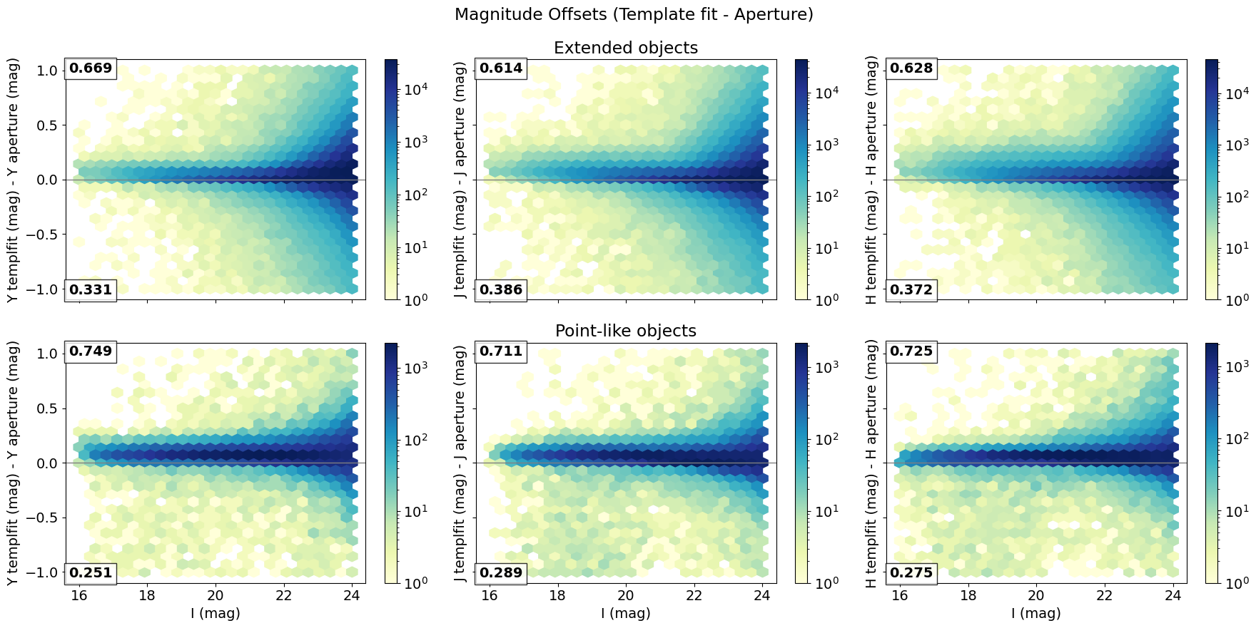
The panel annotations give the fraction of objects with magnitude differences that are positive (top number) and negative (bottom number). The magnitude difference is fairly tightly clustered around 0 for extended objects (top row), but with asymmetric outliers. There is a positive offset, indicating fainter template-fit magnitudes, as expected: templates better exclude contaminating light from nearby sources. The offset is more pronounced for point-like objects (bottom row), likely due to the PSF handling mentioned above, and we are reminded that aperture magnitudes are more reliable here.
About this notebook
Updated: 2025-12-23
Contact: IRSA Helpdesk