Access HATS Collections Using LSDB: Euclid Q1 and ZTF DR23

Learning Goals¶

By the end of this tutorial, you will learn how to:

• Use the lsdb library to access IRSA HATS Collections from the cloud.
• Define spatial, column, and row filters to read only a portion of large HATS catalogs.
• Crossmatch catalogs using lsdb and visualize the results.
• Perform index searches on HATS catalogs using lsdb.

Introduction¶

IRSA provides several astronomical catalogs in spatially partitioned Parquet format, enabling efficient access and scalable analysis of large datasets. Among these are the HATS (Hierarchical Adaptive Tiling Scheme) collections, which organize catalog data using adaptive HEALPix-based partitioning for parallelizable queries and crossmatching.

For more details on HATS collections, partitioning, and schema organization, see the IRSA documentation on Parquet catalogs.

This notebook demonstrates how to access and analyze HATS collections using the lsdb Python library, which makes it convenient to work with these large datasets. We will explore the following IRSA HATS collections in this tutorial:

• Euclid Q1 Merged Objects: 14 Euclid Q1 tables, including MER (multi-wavelength mosaics) final catalog, photometric redshift catalogs, and spectroscopic catalogs joined on MER Object ID.
• ZTF DR23 Objects Table: catalog of PSF-fit photometry detections extracted from ZTF reference images, including “collapsed-lightcurve” metrics.
• ZTF DR23 Lightcurves: catalog of PSF-fit photometry detections extracted from single-exposure images at the locations of Objects Table detections.

We will use lsdb to leverage HATS partitioning for performing fast spatial queries on a relatively large area of sky and for crossmatching sources between Euclid and ZTF to identify variable galaxy candidates and visualize their light curves.

Imports¶

# Uncomment the next line to install dependencies if needed.
# !pip install s3fs "lsdb>=0.6.6" pyarrow pandas numpy astropy dask matplotlib

import s3fs
import lsdb
import pyarrow.parquet as pq
import numpy as np
import pandas as pd
from astropy import units as u
from astropy.coordinates import SkyCoord
import os
import matplotlib.pyplot as plt
from dask.distributed import Client

pd.set_option("display.max_colwidth", None) # schema descriptions can be long
pd.set_option("display.min_rows", 18) # to show more rows when truncated view

1. Locate HATS collections in the cloud¶

From IRSA’s cloud data access page, let’s identify the bucket and path prefix for the HATS Collections for Euclid Q1 and ZTF DR23:

euclid_q1_bucket = "nasa-irsa-euclid-q1"
euclid_q1_hats_prefix = "contributed/q1/merged_objects/hats"

ztf_bucket = "ipac-irsa-ztf"
ztf_hats_prefix = "contributed/dr23/objects/hats"
ztf_lc_hats_prefix = "contributed/dr23/lc/hats"

s3fs provides a filesystem-like Python interface for AWS S3 buckets. First, we create an S3 client:

s3 = s3fs.S3FileSystem(anon=True)

Using the S3 client, we can now list the contents of the Euclid Q1 HATS collection:

s3.ls(f"{euclid_q1_bucket}/{euclid_q1_hats_prefix}")

In this collection, you can see collection properties, catalog, index table, and margin cache in order. You can explore more directories to see how this HATS collection follows the directory structure described in IRSA’s documentation on HATS partitioning and HATS Collections.

As per the documentation, the Parquet file containing the schema for this euclid_q1_merged_objects-hats catalog is stored in dataset/_common_metadata directory. You can find the catalog schema through other sources as well but we use the _common_metadata file here because it contains column metadata (units and descriptions) which the other schemas don’t have. Let’s save its path for later use:

euclid_q1_schema_path = "euclid_q1_merged_objects-hats/dataset/_common_metadata" # euclid_q1_merged_objects-hats is the catalog name we identified above

Similarly, we can list the contents of the ZTF DR23 Objects HATS collection and save the path to its schema file:

s3.ls(f"{ztf_bucket}/{ztf_hats_prefix}")

ztf_schema_path = "ztf_dr23_objects-hats/dataset/_common_metadata" # ztf_dr23_objects-hats is the catalog name we identified above

2. Open the HATS catalogs¶

Now we can use lsdb to open the HATS catalogs we identified above, starting with the Euclid Q1 catalog. Note that we can simply pass the HATS collection path and it will automatically identify the catalog inside it and make use of the ancillary data (index table and margin cache) when needed. Also, we prefix the path with s3:// to indicate that it is an S3 path.

euclid_catalog = lsdb.open_catalog(f"s3://{euclid_q1_bucket}/{euclid_q1_hats_prefix}")
euclid_catalog

Few things to note here:

• This catalog is opened lazily, i.e., no data is read from the S3 bucket into memory yet.
• Since we did not specify any columns to select from this very wide catalog, we get 7 default columns out of 1593 available columns!
• We see some of the HEALPix orders and pixels at which this catalog is partitioned.

Let’s plot the sky coverage of this catalog:

euclid_catalog.plot_pixels()

(<Figure size 1000x500 with 2 Axes>, <WCSAxes: title={'center': 'Catalog pixel map - Euclid_Q1_Merged_Objects'}>)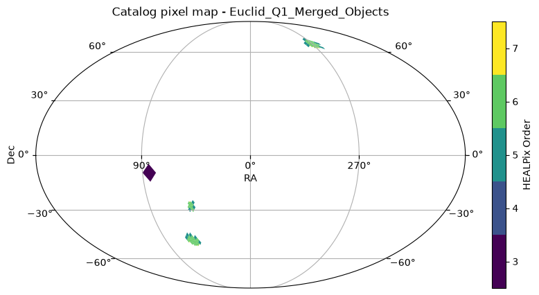

Since HATS uses adaptive tile-based partitioning, we see higher order HEALPix tiles in regions with higher source density and lower order tiles in regions with lower source density.

Now let’s open the ZTF DR23 Objects catalog in a similar manner and view its sky coverage:

ztf_catalog = lsdb.open_catalog(f"s3://{ztf_bucket}/{ztf_hats_prefix}")
ztf_catalog

ztf_catalog.plot_pixels()

(<Figure size 1000x500 with 2 Axes>, <WCSAxes: title={'center': 'Catalog pixel map - ZTF_DR23_Objects'}>)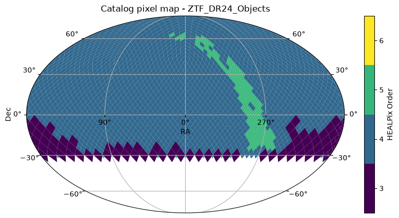

3. Define filters for querying Euclid Q1 catalog¶

3.1 Define a spatial filter¶

From the above two plots, it’s clear that the ZTF DR23 Objects catalog covers a much larger area of the sky compared to the Euclid Q1 catalog. So for cross-matching, we can safely pick the Euclid Deep Field North (EDF-N) region that is covered by both catalogs. From the Euclid user guide at IRSA Table 1, we identify the following for the EDF-N region:

euclid_DF_N_center = SkyCoord('17:58:55.9 +66:01:03.7', unit=('hourangle', 'deg'))
euclid_DF_N_center

# euclid_DF_N_radius = 3 * u.deg  # ceil(sqrt(22.9 / pi)) approximate radius to cover almost entire EDF-N
euclid_DF_N_radius = 0.5 * u.deg  # smaller radius to reduce execution time for this tutorial
euclid_DF_N_radius

Now, using lsdb, we define a cone search object for this region that can be passed as a spatial filter when querying the catalogs:

spatial_filter = lsdb.ConeSearch(
    ra=euclid_DF_N_center.ra.deg, 
    dec=euclid_DF_N_center.dec.deg, 
    radius_arcsec=euclid_DF_N_radius.to(u.arcsec).value
)

We can overplot this spatial filter on the Euclid catalog’s sky coverage to verify (note we limited the field of view so that we can see the cone better):

euclid_catalog.plot_pixels(fov=(8 * u.deg, 6 * u.deg), center=euclid_DF_N_center)
spatial_filter.plot(fc="#00000000", ec="red");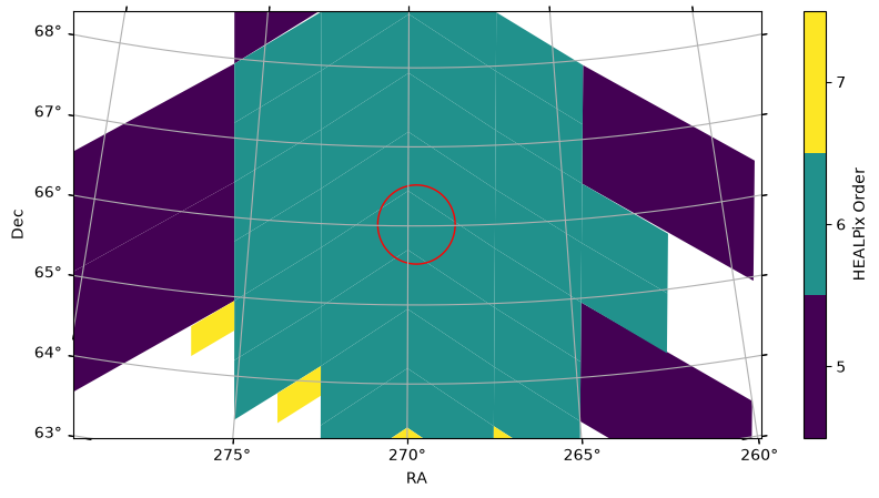

3.2 Identify columns of interest from the schema¶

Before we can define column and row filters for querying any HATS catalog, we need to know what columns are available in that catalog. So let’s inspect the schema of the Euclid Q1 catalog.

Using pyarrow parquet, we can read the schema from the _common_metadata parquet file we identified above (note that we again prefixed the path with s3:// to indicate that it is an S3 path):

euclid_schema = pq.read_schema(
    f"s3://{euclid_q1_bucket}/{euclid_q1_hats_prefix}/{euclid_q1_schema_path}",
    filesystem=s3
)
type(euclid_schema)

Since the schema of this catalog is a pyarrow object, let’s convert it to a pandas DataFrame for easier inspection:

def pq_schema_to_df(schema):
    """Convert a PyArrow schema to a Pandas DataFrame."""
    return pd.DataFrame(
        [
            (
                field.name,
                str(field.type),
                field.metadata.get(b"unit", b"").decode(),
                field.metadata.get(b"description", b"").decode()
            )
            for field in schema # schema is an iterable of pyarrow fields
        ],
        columns=["name", "type", "unit", "description"]
    )

euclid_schema_df = pq_schema_to_df(euclid_schema)
len(euclid_schema_df)

As we saw above, the Euclid HATS catalog contains 1594 columns in its schema!

The columns at the beginning of this schema (such as “tileid”, “objectid”, “ra”, “dec”) define positions and IDs. These can be useful for our column filters — the columns we want to SELECT when querying the catalog.

We can also filter the schema DataFrame by name, unit, type, etc., to identify columns most relevant for our row filters — WHERE rows satisfy conditions on column values for our query. For example, let’s explore the columns that are part of the PHZ (photometric redshift) catalog to identify photometric redshifts and source types:

euclid_schema_df[
    euclid_schema_df["name"].str.startswith("phz_") # phz_ prefix is for PHZ catalog columns in this merged catalog
    & euclid_schema_df["type"].str.contains("int") # to see flag type columns
]

“phz_phz_median” gives us the median photometric redshift of sources, while “phz_phz_classification” can be used to filter the Euclid catalog to only galaxy-type sources.

You can explore the schema DataFrame further to identify any other columns of interest. It is also useful to go through the description of Euclid Q1 data products and papers that contain different PHZ, MER, etc. catalog tables that are merged in this HATS catalog, which are linked in the Euclid Q1 HATS Parquet notebook.

3.3 Define column filters¶

For this tutorial, the following columns are most relevant to us:

euclid_columns = euclid_schema_df['name'].iloc[:7].tolist() # the positional and ID columns
euclid_columns.extend([
    'phz_phz_median', # median of the photometric redshift PDF
])

The selected columns with their metadata are:

euclid_schema_df[euclid_schema_df["name"].isin(euclid_columns)]

3.4 Define row filters¶

To identify the galaxies with quality redshifts in this catalog, the following filters can be applied to the rows (from Tucci et al. 2025 section 5.3):

Note that these filters are defined as lists of lists, where each inner list represents a single condition in the format [column_name, operator, value] and the conditions are combined using logical AND. More on filters that lsdb supports can be found in its documentation.

def magnitude_to_flux(magnitude: float) -> float:
    """Convert magnitude to flux following the MER Photometry Cookbook."""
    zeropoint = 23.9
    flux = 10 ** ((magnitude - zeropoint) / -2.5)
    return flux

galaxy_filters = [
    ['phz_phz_classification', '==', 2], # 2 is for galaxies
    ['mer_vis_det', '==', 1], # No NIR-only objects
    ['mer_spurious_flag', '==', 0], # not spurious
    ['mer_flux_detection_total', '>', magnitude_to_flux(24.5)],  # I < 24.5
    # lsdb doesn't support column arithmetic in filters yet, so can rather apply the S/N > 5 filter after loading the data
    # ['mer_flux_detection_total', '/', 'mer_flux_detection_error_total', '>', 5], # I band S/N > 5
]

4. Define filters for querying ZTF DR23 Objects catalog¶

Since we are interested in cross-matching ZTF DR23 Objects with the Euclid Q1 catalog, we will use the same spatial filter defined above.

We can define column and row filters for the ZTF catalog based on its schema, similar to the previous section:

ztf_schema = pq.read_schema(
    f"s3://{ztf_bucket}/{ztf_hats_prefix}/{ztf_schema_path}",
    filesystem=s3
)
ztf_schema_df = pq_schema_to_df(ztf_schema)

You can filter the schema further by units, type, etc. to identify other columns of interest. It’s also useful to go through the ZTF DR23 release notes and explanatory supplement at IRSA for more details on column selections and caveats.

For this tutorial, the following columns are most relevant to us:

ztf_columns = ztf_schema_df["name"].tolist()[:6]
ztf_columns.extend([
    'fid', 'filtercode', 
    'ngoodobsrel',  
    'chisq', 'magrms', 'meanmag', 'medianabsdev'
])

The rationale for selecting these columns is as follows:

ztf_schema_df[ztf_schema_df.name.isin(ztf_columns)]

For a quality cut, we apply the following filter on the number of good epochs (from Coughlin et al. 2021 section 2):

quality_filters = [
    ["ngoodobsrel", ">", 50]
]

5. Crossmatch: Euclid Q1 x ZTF DR23 Objects¶

Now that we have defined the spatial, column, and row filters for both catalogs, we can use lsdb to perform the crossmatch.

5.1 Create crossmatch query using the filters¶

Following lsdb’s documentation on performing filters, we open the Euclid Q1 catalog with the defined spatial, column, and row filters:

euclid_cone = lsdb.open_catalog(
    f"s3://{euclid_q1_bucket}/{euclid_q1_hats_prefix}",
    columns=euclid_columns,
    search_filter=spatial_filter,
    filters=galaxy_filters
)
euclid_cone

Notice how the number of partitions reduced from 114 (in section 2) to only a few partitions that are within the spatial filter. This allows LSDB to avoid loading unused parts of the catalog. Also, we see only the columns we selected in the column filters.

Now, similarly, we open the ZTF DR23 Objects catalog with its defined filters:

ztf_cone = lsdb.open_catalog(
    f"s3://{ztf_bucket}/{ztf_hats_prefix}",
    columns=ztf_columns,
    search_filter=spatial_filter,
    filters=quality_filters
)
ztf_cone

We see a similar reduction in the number of partitions for this catalog as well, and our column selection is applied.

Now we can use lsdb’s crossmatch functionality to plan a crossmatch between these two filtered catalogs. Note that the order of crossmatch matters: lsdb’s algorithm takes each object in the left catalog and finds the closest spatial match from the right catalog. Since Euclid is denser than ZTF, we put it on the left side of the crossmatch to maximize the number of matches. For more details on the parameters, refer to the documentation linked.

euclid_x_ztf = euclid_cone.crossmatch(
    ztf_cone,
    suffixes=("_euclid", "_ztf"), # to distinguish columns from the two catalogs
    n_neighbors=1, # default is 1 too, can be tweaked
    radius_arcsec=1  # default is 1 arcsec too, can be tweaked
)
euclid_x_ztf

Note how the resulting crossmatched catalog contains columns from both catalogs with the suffixes we passed. As we noticed when opening the catalog, this created a crossmatch catalog object lazily but did not execute the crossmatch.

5.2 Execute the query and load data¶

Now we can run the crossmatch query we have been planning so far by using the compute() method of the crossmatch catalog object, which will perform all the tasks and return the result as a DataFrame. lsdb utilizes Dask to parallelize the tasks on different partitions, so we need to create a Dask client to manage the resources (and track progress) for the scope of this computation:

def get_nworkers(catalog):
    return min(os.cpu_count(), catalog.npartitions + 1)

with Client(n_workers=get_nworkers(euclid_x_ztf), 
            threads_per_worker=2, 
            memory_limit='auto') as client:
    print(f"This may take more than a few minutes to complete. You can monitor progress in Dask dashboard at {client.dashboard_link}")
    euclid_x_ztf_df = euclid_x_ztf.compute() # this will load the data into memory finally

This may take more than a few minutes to complete. You can monitor progress in Dask dashboard at http://127.0.0.1:8787/status

euclid_x_ztf_df

5.3 Identify objects of interest from the crossmatch¶

Check the number of unique Euclid and ZTF sources in the crossmatched catalog:

euclid_x_ztf_df.shape[0], euclid_x_ztf_df['object_id_euclid'].nunique(), euclid_x_ztf_df['oid_ztf'].nunique()

This means there is one unique Euclid source for each row in the crossmatched catalog as expected (since we put Euclid on the left side of the crossmatch). But for ZTF, this is not true as some ZTF objects have multiple Euclid matches since ZTF has lower resolution than Euclid.

Now let’s plot some variability metrics from ZTF against Euclid redshift to see if there are any trends. We will use hexbin plots to visualize the density of sources in each panel:

z = euclid_x_ztf_df["phz_phz_median_euclid"].to_numpy() # x-axis
metrics = [ # y-axes
    ("magrms_ztf",        "ZTF mag RMS"),
    ("chisq_ztf",         "ZTF χ²"),
    ("medianabsdev_ztf",  "ZTF MAD"),
    ("ngoodobsrel_ztf",   "ZTF # good obs"),
]

fig, axes = plt.subplots(2, 2, figsize=(10, 6), constrained_layout=True, sharex=True)
axes = axes.ravel()

xmin, xmax = 0, 2.5  
gridsize = 48  # resolution: larger => finer grid

for i, (col, ylabel) in enumerate(metrics):
    ax = axes[i]
    y = euclid_x_ztf_df[col].to_numpy()

    # clip y to robust range (1–99th percentile) for visibility
    y_lo, y_hi = np.nanpercentile(y, [1, 99])

    hb = ax.hexbin(
        z, y,
        gridsize=gridsize,
        extent=(xmin, xmax, y_lo, y_hi),
        mincnt=1,
        bins='log'  # logarithmic color scale of counts
    )

    # ax.set_xlim(xmin, xmax)
    # ax.set_ylim(y_lo, y_hi)
    ax.set_ylabel(ylabel)

    # x-label only on bottom row to reduce clutter
    if i // 2 == 1:
        ax.set_xlabel("Euclid redshift")


# Shared colorbar across all panels (uses last hexbin as mappable)
cbar = fig.colorbar(hb, ax=axes[:-1], shrink=0.9, label="Galaxy sources count (log)")

fig.suptitle("Euclid redshift vs ZTF variability metrics", y=1.04)
plt.show()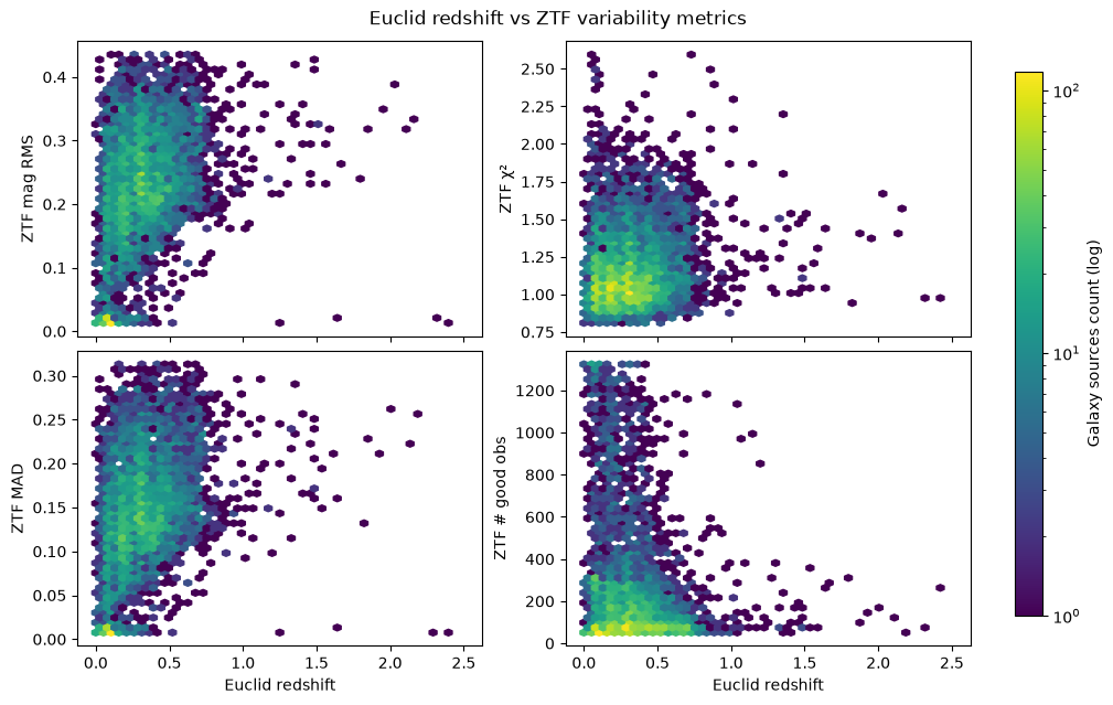

There’s no strong variability trend for higher redshift galaxies (z > 1) as the distributions of mag RMS, MAD, and Chi-squared are fairly stable with redshift. This is likely because of the limited sensitivity of ZTF, as there are clearly fewer good observations as redshift increases.

Despite this, we can still select some high-variability galaxy sources from the low redshift (z < 1) range for further analysis. Let’s focus only on Chi-squared (measure of significance) and RMS magnitude (measure of variability amplitude; similar to MAD) metrics:

euclid_x_ztf_df['chisq_ztf'].describe()

chisq_threshold = euclid_x_ztf_df['chisq_ztf'].quantile(0.95)
chisq_threshold

euclid_x_ztf_df['magrms_ztf'].describe()

magrms_threshold = euclid_x_ztf_df['magrms_ztf'].quantile(0.95)
magrms_threshold

variable_galaxies = euclid_x_ztf_df.query(
    f"chisq_ztf >= {chisq_threshold} & magrms_ztf >= {magrms_threshold}"
    ).sort_values("chisq_ztf", ascending=False) # sort by significant variability

Let’s inspect the top variable galaxies that we can use for plotting their light curves:

cols_of_interest = ["oid_ztf", "fid_ztf", "filtercode_ztf", "phz_phz_median_euclid", "magrms_ztf", "chisq_ztf"]
top_variable_galaxies = variable_galaxies.head(3)
top_variable_galaxies[cols_of_interest]

6. Load ZTF lightcurves by object IDs¶

Let’s open the ZTF light curves HATS catalog. Note that we are using the same spatial filter as before. We do not specify any column filters, because the default columns already contain the light curve data we need. We also do not apply any row filters, since we will directly filter rows by object IDs.

ztf_lc_catalog = lsdb.open_catalog(f"s3://{ztf_bucket}/{ztf_lc_hats_prefix}",
                                   search_filter=spatial_filter
                                   )
ztf_lc_catalog

We can inspect the catalog’s collection properties and find which columns have ancillary index tables (as explained in lsdb’s documentation on using index tables).

ztf_lc_idx_column = list(ztf_lc_catalog.hc_collection.all_indexes.keys())[0]
ztf_lc_idx_column

Let’s just extract the object IDs of the top variable galaxies we identified above:

ztf_oids = top_variable_galaxies['oid_ztf'].tolist()
ztf_oids

Now we can use these IDs to filter the ZTF light curves catalog by the id_search method:

ztf_lcs = ztf_lc_catalog.id_search(values={ztf_lc_idx_column: ztf_oids})
ztf_lcs

As earlier, this creates a lazy catalog object with the partition(s) that contains our IDs. We can load the light curves data into a DataFrame by using the compute() method:

ztf_lcs_df = ztf_lcs.compute() # ID search runs out of memory if we try to parallelize it with Dask client
ztf_lcs_df

Let’s merge this light curves DataFrame with the crossmatched catalog (with variability filters and sorting) so that we can use collapsed light curves metrics for annotating the plots:

merged_ztf_lcs_df = ztf_lcs_df.merge(
    top_variable_galaxies[cols_of_interest].set_index('oid_ztf'),
    left_on='objectid', right_index=True
).set_index('objectid', drop=False)

# Sort by the order of top_variable_galaxies
merged_ztf_lcs_df = merged_ztf_lcs_df.loc[ztf_oids]
merged_ztf_lcs_df

Now we can finally plot the light curves of these variable galaxy candidates. We need to filter out bad epochs using the catflags column as explained in the ZTF DR23 explanatory supplement section 13.6. Then, we will plot the light curves in separate panels for each object:

fig, axs = plt.subplots(len(merged_ztf_lcs_df), 1, figsize=(10, 4 * len(merged_ztf_lcs_df)), constrained_layout=True)

if len(merged_ztf_lcs_df) == 1:
    axs = [axs]

for ax, (_, row) in zip(axs, merged_ztf_lcs_df.iterrows()):
    lc = row['lightcurve'].query("catflags == 0")  # remove bad epochs
    lc_label = (f'ZTF DR23 Object {row["objectid"]} in band {row["filtercode_ztf"][1]}\n'
                f'(z={row["phz_phz_median_euclid"]:.2f}, RMS mag={row["magrms_ztf"]:.3f}, Chi-sq={row["chisq_ztf"]:.3f})')
    pts = ax.plot(lc['hmjd'], lc['mag'], '.', markersize=4, label=lc_label, zorder=3)
    ax.errorbar(
        lc['hmjd'], lc['mag'], yerr=lc['magerr'],
        fmt='none', ecolor=pts[0].get_color(), elinewidth=0.8, capsize=0, alpha=0.3, zorder=2
    )
    ax.set_ylabel('Magnitude')
    ax.set_xlabel('HMJD')
    ax.invert_yaxis()
    ax.set_title(lc_label, fontsize=10)

fig.suptitle("Lightcurves of Variable Galaxy Candidates", fontsize=14, y=1.02)
fig.set_constrained_layout_pads(h_pad=0.15)
plt.show()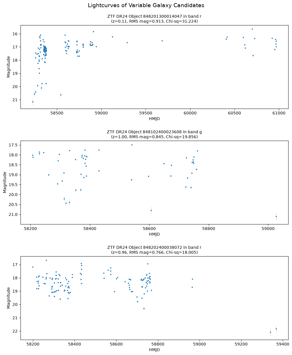

About this notebook¶

Author: Jaladh Singhal, Troy Raen, Jessica Krick, Brigitta Sipőcz, Vandana Desai, and the IRSA Data Science Team

Updated: 2025-10-02

Contact: the IRSA Helpdesk with questions or to report problems.