Searching for AllWISE Images with SIA v2

Learning Goals¶

By the end of this tutorial, you will:

• Learn how to access IRSA’s WISE AllWISE Atlas (L3a) coadded images via the Simple Image Access (SIA) service.

• Identify which of IRSA’s AllWISE Atlas images cover a specified coordinate.

• Visualize one of the identified images using Firefly.

• Create and display a cutout of the downloaded image.

Introduction¶

The AllWISE program builds upon the work of the successful Wide-field Infrared Survey Explorer mission (WISE; Wright et al. 2010) by combining data from the WISE cryogenic and NEOWISE (Mainzer et al. 2011 ApJ, 731, 53) post-cryogenic survey phases to form the a comprehensive view of the full mid-infrared sky. The AllWISE Images Atlas is comprised of 18,240 4-band calibrated 1.56°x1.56° FITS images, depth-of-coverage and noise maps, and image metadata produced by coadding nearly 7.9 million Single-exposure images from all survey phases. For more information about the WISE mission, see:

https://irsa.ipac.caltech.edu/Missions/wise.html

The NASA/IPAC Infrared Science Archive (IRSA) at Caltech is the archive for AllWISE images and catalogs. The AllWISE Atlas images that are the subject of this tutorial are made accessible via the International Virtual Observatory Alliance (IVOA) Simple Image Access (SIA) protocol.

Imports¶

• numpy for working with tables

• astropy.coordinates for defining coordinates

• astropy.nddata for creating an image cutout

• astropy.wcs for interpreting the World Coordinate System header keywords of a fits file

• astropy.units for attaching units to numbers passed to the SIA service

• matplotlib.pyplot for plotting

• astropy.io to manipulate FITS files

• firefly_client for visualizing images

• astroquery.ipac.irsa for IRSA data access

• astropy.visualization for color stretch display

# Uncomment the next line to install dependencies if needed.
# %pip install matplotlib astropy astroquery jupyter_firefly_extensions

import numpy as np
from astropy.coordinates import SkyCoord
from astropy.nddata import Cutout2D
from astropy.wcs import WCS
import astropy.units as u
import matplotlib.pyplot as plt
from astropy.io import fits
from firefly_client import FireflyClient
from astroquery.ipac.irsa import Irsa
from astropy.visualization import simple_norm

1. Define the target¶

Define coordinates of a bright star

ra = 314.30417
dec = 77.595559
pos = SkyCoord(ra=ra, dec=dec, unit='deg')

2. Discover AllWISE Atlas images¶

IRSA provides Simple Image Access (SIA) services for various datasets. A list of available datasets and their access URLs can be found here. This tutorial uses SIA v2 for AllWISE Atlas images. To search for other datasets on SIA v2, try changing the filter string. Or remove the filter keyword altogether to get a full list of available SIA v2 datasets at IRSA.

First we need to know the name of the dataset on the IRSA system.

names = Irsa.list_collections(filter="allwise")
names

We see from the resulting table that the dataset collection we are interested in is called “wise_allwise”. Use this collection name in query below.

3. Search for images¶

Which images in the IRSA allwise dataset include our target of interest?

Get a table of all images within 1 arcsecond of our target position.

im_table = Irsa.query_sia(pos=(pos, 1 * u.arcsec), collection='wise_allwise')

Inspect the table that is returned.

im_table

Look at a list of the column names included in this table.

im_table.colnames

Look at the unique values in one of the columns.

print(np.unique(im_table['energy_bandpassname']))

energy_bandpassname
-------------------
                 W1
                 W2
                 W3
                 W4

4.Locate and visualize an image of interest¶

We start by filtering the image results for the W3 band images. Then look at the header of one of the resulting W3 band images of our target star. Finally, we create an interactive FITS display of the W3 image(s) by using Firefly, an open-source interactive visualization tool for astronomical data. To understand how to open the Firefly viewer in a new tab from your Python notebook, refer to this documentation on how to initialize FireflyClient.

You can put the URL from the column “access_url” into a browser to download the file. Or you can work with it in Python, as shown below.

w3_mask = im_table['energy_bandpassname'] == 'W3'
w3_table = im_table[w3_mask]

Lets look at the access_url of the first one. Then use Astropy to examine the header of the URL from the previous step, and grab the data and wcs from the header.

image_url = w3_table['access_url'][0]
image_url

with fits.open(image_url, memmap=False) as hdul:
    hdul.info()
    data = hdul[0].data
    wcs = WCS(hdul[0].header)

Filename: /home/runner/.astropy/cache/download/url/8d2ca559dab02f02cfae68b955dcbad3/contents
No.    Name      Ver    Type      Cards   Dimensions   Format
  0  PRIMARY       1 PrimaryHDU      71   (4095, 4095)   float32   

Visualize an image by sending its URL to the Firefly viewer. Try using the interactive tools in the viewer to explore the data.

# Uncomment when opening a Firefly viewer in a tab within Jupyter Lab with jupyter_firefly_extensions installed
# fc = FireflyClient.make_lab_client()

# Uncomment when opening Firefly viewer in contexts other than the above
fc = FireflyClient.make_client(url="https://irsa.ipac.caltech.edu/irsaviewer")

# Visualize an image by sending its URL to the viewer.
fc.show_fits_image(file_input=image_url,
             plot_id="image",
             Title="Image"
             )

5. Extract a cutout and plot it¶

If you want to see just a cutout of a certain region around the target, we do that below using astropy’s Cutout2D.

# make 1' x 1' cutout
cutout = Cutout2D(data, position=pos, size=1 * u.arcmin, wcs=wcs)

#add quick normalization/stretch
norm = simple_norm(cutout.data, stretch="sqrt", percent=99)

# display
plt.imshow(cutout.data, origin='lower', norm = norm)
plt.colorbar(label="Image value")
plt.title("ALLWISE W3 (quicklook)")
plt.xlabel("Pixel X")
plt.ylabel("Pixel Y")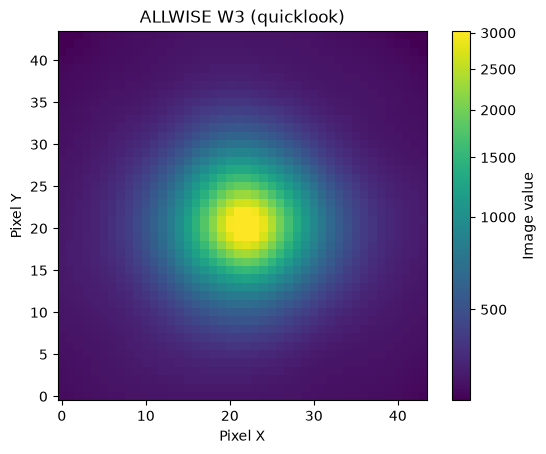

Acknowledgements¶

• Caltech/IPAC-IRSA

About this notebook¶

Updated: 2 March 2026

Contact: IRSA Helpdesk with questions or problems.

Runtime: As of the date above, this notebook takes about 20 seconds to run to completion on a machine with 8GB RAM and 4 CPU. This runtime is dependent on archive servers which means runtime will vary for users.

Citations¶

Astropy: This work made use of Astropy a community-developed core Python package and an ecosystem of tools and resources for astronomy (Astropy Collaboration et al., 2013, Astropy Collaboration et al., 2018, Astropy Collaboration et al.,2022).

Astroquery: This work made use of Astroquery a set of tools for querying astronomical web forms and databases (Ginsburg, Sipőcz, Brasseur et al 2019.).

WISE: This publication makes use of data products from the Wide-field Infrared Survey Explorer, which is a joint project of the University of California, Los Angeles, and the Jet Propulsion Laboratory/California Institute of Technology, funded by the National Aeronautics and Space Administration." Digital Object Identifier (DOI): WISE team (2020)