Searching for contributed COSMOS images

This notebook tutorial demonstrates the process of querying IRSA’s Simple Image Access (SIA) service for the COSMOS images, making a cutout image (thumbnail), and displaying the cutout.

Learning Goals¶

By the end of this tutorial, you will:

• Learn how to search the NASA Astronomical Virtual Observatory Directory web portal for a service that provides access to IRSA’s COSMOS images.
• Use the Python pyvo package to identify which of IRSA’s COSMOS images cover a specified coordinate.
• Download one of the identified images.
• Create and display a cutout of the downloaded image.

Introduction¶

The COSMOS Archive serves data taken for the Cosmic Evolution Survey with HST (COSMOS) project, using IRSA’s general search service, Atlas. COSMOS is an HST Treasury Project to survey a 2 square degree equatorial field with the ACS camera. For more information about COSMOS, see:

https://irsa.ipac.caltech.edu/Missions/cosmos.html

The NASA/IPAC Infrared Science Archive (IRSA) at Caltech is one of the archives for COSMOS images and catalogs. The COSMOS images that are the subject of this tutorial are made accessible via the International Virtual Observatory Alliance (IVOA) Simple Image Access (SIA) protocol. IRSA’s SEIP SIA service is registered in the NASA Astronomical Virtual Observatory (NAVO) Directory. Based on the registered information, the Python package pyvo can be used to query the SIA service for a list of images that meet specified criteria, and standard Python libraries can be used to download and manipulate the images. Other datasets at IRSA are available through other SIA services:

https://irsa.ipac.caltech.edu/docs/program_interface/api_images.html

Imports¶

• pyvo for querying IRSA’s COSMOS SIA service
• astropy.coordinates for defining coordinates
• astropy.nddata for creating an image cutout
• astropy.wcs for interpreting the World Coordinate System header keywords of a fits file
• astropy.units for attaching units to numbers passed to the SIA service
• matplotlib.pyplot for plotting
• astropy.utils.data for downloading files
• astropy.io to manipulate FITS files

# Uncomment the next line to install dependencies if needed.
# !pip install matplotlib astropy pyvo

import pyvo as vo
from astropy.coordinates import SkyCoord
from astropy.nddata import Cutout2D
from astropy.wcs import WCS
import astropy.units as u
import matplotlib.pyplot as plt
from astropy.utils.data import download_file
from astropy.io import fits

Section 1 - Setup¶

Set images to display in the notebook

%matplotlib inline

Define coordinates of a bright source

ra = 149.99986
dec = 2.24875
pos = SkyCoord(ra=ra, dec=dec, unit='deg')

Section 2 - Lookup and define a service for COSMOS images¶

Start at STScI VAO Registry at https://vao.stsci.edu/keyword-search/

Limit by Publisher “NASA/IPAC Infrared Science Archive” and Capability Type “Simple Image Access Protocol” then search on “COSMOS”

Locate the SIA2 URL https://irsa.ipac.caltech.edu/cgi-bin/Atlas/nph-atlas?mission=COSMOS&hdr_location=\COSMOSDataPath\&collection_desc=Cosmic+Evolution+Survey+with+HST+(COSMOS)&SIAP_ACTIVE=1&

cosmos_service = vo.dal.SIAService("https://irsa.ipac.caltech.edu/cgi-bin/Atlas/nph-atlas?mission=COSMOS&hdr_location=%5CCOSMOSDataPath%5C&collection_desc=Cosmic+Evolution+Survey+with+HST+%28COSMOS%29&SIAP_ACTIVE=1&")

Section 3 - Search the service¶

Search for images covering within 1 arcsecond of the star

im_table = cosmos_service.search(pos=pos, size=1.0*u.arcsec)

Inspect the table of images that is returned

im_table

im_table.to_table().colnames

View the first ten entries of the table

im_table.to_table()[:10]

Section 4 - Locate and download an image of interest¶

Locate the first image in the band_name of i+

for i in range(len(im_table)):
    if im_table[i]['band_name'] == 'i+':
        break
print(im_table[i].getdataurl())

https://irsa.ipac.caltech.edu:443/data/COSMOS/images/subaru/best_psf/ip/subaru_ip_best-psf_066_rms_20.fits

Download the image

fname = download_file(im_table[i].getdataurl(), cache=True)
image1 = fits.open(fname)

Section 5 - Extract a cutout and plot it¶

wcs = WCS(image1[0].header)

Make a cutout centered on the position

cutout = Cutout2D(image1[0].data, pos, (60, 60), wcs=wcs)
wcs = cutout.wcs

fig = plt.figure()

ax = fig.add_subplot(1, 1, 1, projection=wcs)
ax.imshow(cutout.data, cmap='gray_r', origin='lower')
ax.scatter(ra, dec, transform=ax.get_transform('fk5'), s=500, edgecolor='red', facecolor='none')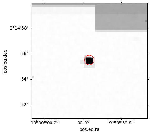

About this notebook¶

Author: David Shupe, IRSA Scientist, and the IRSA Science Team

Updated: 2022-02-14

Contact: the IRSA Helpdesk with questions or reporting problems.

Citations¶

If you use astropy for published research, please cite the authors. Follow these links for more information about citing astropy:

• Citing astropy

If you use COSMOS ACS imaging data in published research, please cite the dataset Digital Object Identifier (DOI): COSMOS Project (2020).