Access ZTF DR24 Light Curves from HATS Catalog

Learning Goals¶

By the end of this tutorial, you will learn how to:

• Open ZTF DR24 Lightcurves and Objects Table HATS Catalogs using lsdb.

• Retrieve light curves for specific objects by ZTF object IDs using an index search.

• Retrieve light curves for objects in a sky region using a cone search.

• Cross-reference the Objects Table to enrich cone search results with per-object variability statistics.

• Plot ZTF light curves (filtered by variability statistics).

Introduction¶

The ZTF DR24 enhanced data products at IRSA include two HATS (Hierarchical Adaptive Tiling Scheme) catalogs hosted on AWS S3:

• Lightcurves catalog: one row per ZTF object, with a nested column storing the full photometry time series — timestamps, magnitudes, uncertainties, and quality flags.

• Objects Table: one row per ZTF object, with collapsed light curve metrics such as magnitude RMS, chi-squared variability statistic, number of good observations, and mean magnitude.

These HATS catalogs offer a scalable, cloud-native alternative to the ZTF light curve service, enabling efficient access especially when the service is overloaded. The lsdb Python library provides a convenient interface for working with HATS catalogs, including spatial queries and object-ID-based lookups.

This tutorial covers two common entry points for accessing ZTF light curves:

1. Object IDs: you have specific ZTF object IDs — from a previous query, a catalog crossmatch, or a published object list — and want their light curves directly.

2. RA/Dec: you have sky coordinates and want all ZTF objects within a given radius.

Both approaches are demonstrated below. An optional section then shows how to join the position search results with the Objects Table to select and plot the most variable objects using robust variability statistics.

For more context on ZTF DR24 data products, refer to the ZTF DR24 release notes and explanatory supplement at IRSA.

Imports¶

# Uncomment the next line to install dependencies if needed.
# !pip install s3fs "lsdb>=0.8.1" pyarrow pandas astropy matplotlib

import s3fs
import lsdb
import pyarrow.parquet as pq
from astropy.coordinates import SkyCoord
import pandas as pd
from astropy import units as u
import os
import matplotlib.pyplot as plt
from dask.distributed import Client

/home/runner/work/irsa-tutorials/irsa-tutorials/.tox/py312-buildhtml/lib/python3.12/site-packages/tqdm/auto.py:21: TqdmWarning: IProgress not found. Please update jupyter and ipywidgets. See https://ipywidgets.readthedocs.io/en/stable/user_install.html
  from .autonotebook import tqdm as notebook_tqdm

pd.set_option("display.max_colwidth", None)
pd.set_option("display.min_rows", 18)

1. Locate ZTF DR24 HATS Catalogs in the Cloud¶

From IRSA’s cloud data access page, we identify the S3 bucket and path prefixes for the ZTF DR24 HATS catalogs:

ztf_bucket = "ipac-irsa-ztf"
ztf_lc_hats_prefix = "ztf/enhanced/dr24/lc/hats" # Lightcurves catalog
ztf_objects_hats_prefix = "ztf/enhanced/dr24/objects/hats" # Objects Table

s3fs provides a filesystem-like Python interface for AWS S3 buckets. First, we create an S3 client:

s3 = s3fs.S3FileSystem(anon=True)

Let’s list the contents of the ZTF DR24 Lightcurves HATS Collection:

s3.ls(f"{ztf_bucket}/{ztf_lc_hats_prefix}")

In this collection, you can see collection properties, catalog, index table, and margin cache in order. You can explore more directories to see how this HATS Collection follows the directory structure described in IRSA’s documentation on HATS partitioning and HATS Collections.

As per the documentation, the Parquet file containing the schema for this catalog is stored in dataset/_common_metadata. Let’s save its path for later use (using the catalog name identified from the listing above):

ztf_lc_schema_path = "ztf_dr24_lc-hats/dataset/_common_metadata"  # ztf_dr24_lc-hats is the catalog name identified above

Similarly, let’s list the ZTF DR24 Objects Table HATS Collection:

s3.ls(f"{ztf_bucket}/{ztf_objects_hats_prefix}")

ztf_objects_schema_path = "ztf_dr24_objects-hats/dataset/_common_metadata"  # ztf_dr24_objects-hats is the catalog name identified above

2. Explore the Catalog Schema¶

Before querying the catalogs, let’s inspect what columns are available in each. We read schemas from the _common_metadata files, which also contain column metadata such as units and descriptions:

def pq_schema_to_df(schema):
    """Convert a PyArrow schema to a Pandas DataFrame."""
    return pd.DataFrame(
        [
            (
                field.name,
                str(field.type),
                field.metadata.get(b"unit", b"").decode(),
                field.metadata.get(b"description", b"").decode()
            )
            for field in schema
        ],
        columns=["name", "type", "unit", "description"]
    )

ztf_lc_schema = pq.read_schema(
    f"s3://{ztf_bucket}/{ztf_lc_hats_prefix}/{ztf_lc_schema_path}",
    filesystem=s3
)
ztf_lc_schema_df = pq_schema_to_df(ztf_lc_schema)
ztf_lc_schema_df

Notice the lightcurve column — this is a nested column that stores the full photometric time series for each ZTF object. Each element of lightcurve is itself a table with columns including hmjd, mag,magerr, clrcoeff and catflags. We save the list of columns interesting to us for later use when opening the catalog with lsdb:

ztf_lc_columns = ["objectid", "objra", "objdec", "filterid", "nepochs", "lightcurve"]

3. Get Light Curves by Object ID¶

If you have specific ZTF object IDs, you can retrieve their light curves directly using an index search — no spatial filter needed. This is the fastest approach for targeted lookups.

3.1 Open the Lightcurves Catalog¶

We open the ZTF DR24 Lightcurves HATS catalog. No data is read yet — lsdb opens catalogs lazily:

ztf_lc_catalog = lsdb.open_catalog(
    f"s3://{ztf_bucket}/{ztf_lc_hats_prefix}",
    columns=ztf_lc_columns
)
ztf_lc_catalog

3.2 Identify the Index Column¶

The ZTF DR24 Lightcurves HATS catalog ships with an ancillary index table that enables fast lookups by object ID. Let’s identify which column is indexed:

ztf_lc_idx_column = list(ztf_lc_catalog.hc_collection.all_indexes.keys())[0]
print(f"Index column: {ztf_lc_idx_column}")

Index column: objectid

3.3 Perform an Index Search¶

We use the same object IDs from the ZTF light curve API docs multi-object example — you can compare results from this tutorial directly with that service. In your workflow, these IDs might come from a previous query, a catalog crossmatch, or a published object catalog:

object_ids = [686103400034440, 686103400106565]

ztf_lcs_by_id = ztf_lc_catalog.id_search(values={ztf_lc_idx_column: object_ids})
ztf_lcs_by_id

Searching for objectid=[686103400034440, 686103400106565]

3.4 Compute and Inspect the Results¶

Now we execute the query by calling compute(), which reads the data into memory as a Pandas DataFrame. We use a Dask client to parallelize across partitions, manage memory, and monitor progress in the Dask dashboard.

def get_nworkers(catalog):
    return min(os.cpu_count(), catalog.npartitions + 1)

with Client(n_workers=get_nworkers(ztf_lcs_by_id),
            threads_per_worker=1,
            memory_limit=None  # each partition can be several GB; avoid per-worker cap
            ) as client:
    print(f"You can monitor progress in the Dask dashboard at {client.dashboard_link}")
    ztf_lcs_by_id_df = ztf_lcs_by_id.compute()

ztf_lcs_by_id_df

You can monitor progress in the Dask dashboard at http://127.0.0.1:8787/status

2026-07-11 00:42:31,564 - distributed.nanny - WARNING - Worker process still alive after 4.0 seconds, killing

print(f"Found {len(ztf_lcs_by_id_df)} light curves for {len(object_ids)} objects.")

Found 2 light curves for 2 objects.

Each row is one ZTF object. The lightcurve column contains a nested DataFrame per object. Let’s inspect the light curve of the first object:

ztf_lcs_by_id_df['lightcurve'].iloc[0]

3.5 Plot Light Curves¶

When plotting the light curves, it’s important to note that we apply catflags == 0 filter to keep only clean epochs (as described in the explanatory supplement section 13.6).

fig, axs = plt.subplots(len(ztf_lcs_by_id_df), 1,
                        figsize=(10, 4 * len(ztf_lcs_by_id_df)),
                        constrained_layout=True)

if len(ztf_lcs_by_id_df) == 1:
    axs = [axs]

for ax, (_, row) in zip(axs, ztf_lcs_by_id_df.iterrows()):
    lc = row['lightcurve'].query("catflags == 0")  # to keep only clean epochs
    title = f"ZTF Object {row['objectid']}  (RA={row['objra']:.4f}°, Dec={row['objdec']:.4f}°)"
    pts = ax.plot(lc['hmjd'], lc['mag'], '.', markersize=4, zorder=3)
    ax.errorbar(
        lc['hmjd'], lc['mag'], yerr=lc['magerr'],
        fmt='none', ecolor=pts[0].get_color(), elinewidth=0.8, alpha=0.3, zorder=2
    )
    ax.set_ylabel("Magnitude")
    ax.set_xlabel("HMJD")
    ax.invert_yaxis()
    ax.set_title(title, fontsize=10)

fig.suptitle("ZTF DR24 Light Curves — Object ID Search Results", fontsize=13, y=1.02)
plt.show()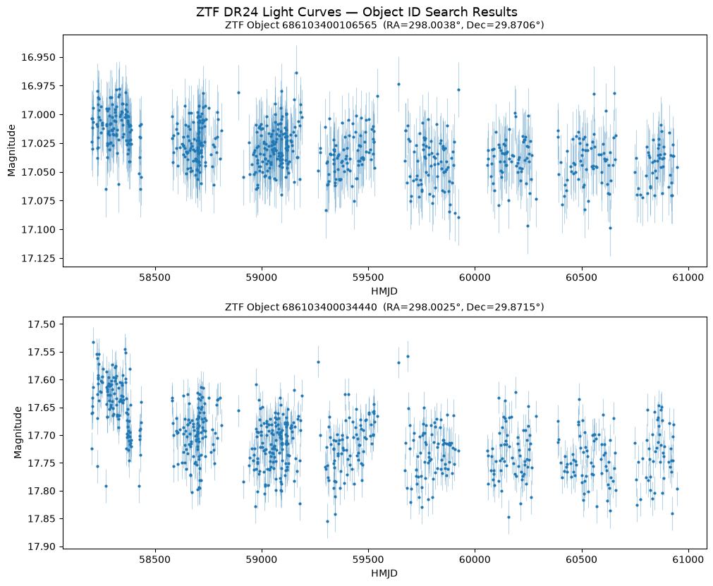

4. Get Light Curves by Sky Position¶

If you have sky coordinates and want all ZTF objects within a given area, use a spatial search. We’ll do a cone search here. Box and polygon searches are also available.

4.1 Define a Spatial Filter¶

We use the same sky position as the ZTF light curve API docs positional example but you can specify any coordinates and search radius you want:

target = SkyCoord(ra=298.0025, dec=29.87147, unit="deg")
search_radius = 1 * u.arcsec # to keep the runtime minimal for this tutorial

Using lsdb, we define a cone search object for this region:

spatial_filter = lsdb.ConeSearch(
    ra=target.ra.deg,
    dec=target.dec.deg,
    radius_arcsec=search_radius.to(u.arcsec).value
)

4.2 Define Row Filters¶

In addition to the spatial filter, we can pre-filter rows using Parquet column statistics. Here we keep only objects with more than 25 epochs, focusing on well-sampled light curves:

row_filters = [
    ["nepochs", ">", 25],
    # additional filters can be added here if desired
    ]

4.3 Open the Filtered Lightcurves Catalog¶

We open the catalog with both filters applied. lsdb evaluates this lazily — no data is read yet:

ztf_lc_cone = lsdb.open_catalog(
    f"s3://{ztf_bucket}/{ztf_lc_hats_prefix}",
    search_filter=spatial_filter,
    columns=ztf_lc_columns,
    filters=row_filters
)
ztf_lc_cone

Notice that only the partitions overlapping the cone are included, avoiding reads of the full catalog.

4.4 Compute and Inspect the Results¶

Now we execute the query by calling compute(), which reads the data into memory as a Pandas DataFrame. We use a Dask client to parallelize across partitions, manage memory, and monitor progress in the Dask dashboard.

with Client(n_workers=get_nworkers(ztf_lc_cone),
            threads_per_worker=1,
            memory_limit=None  # each partition can be several GB; avoid per-worker cap
            ) as client:
    print(f"You can monitor progress in the Dask dashboard at {client.dashboard_link}")
    ztf_lc_cone_df = ztf_lc_cone.compute()

You can monitor progress in the Dask dashboard at http://127.0.0.1:8787/status

print(f"Found {len(ztf_lc_cone_df)} ZTF light curves for the search criteria.")

Found 5 ZTF light curves for the search criteria.

ztf_lc_cone_df.head(5)

Each row corresponds to one ZTF object. The lightcurve column contains a nested DataFrame per object:

ztf_lc_cone_df['lightcurve'].iloc[0]

5. [Optional] Look Up Additional Info from the Objects Table¶

5.1 Explore the Objects Table Schema¶

The Objects Table contains summary statistics for each ZTF object. Let’s inspect its schema to identify columns of interest:

ztf_objects_schema = pq.read_schema(
    f"s3://{ztf_bucket}/{ztf_objects_hats_prefix}/{ztf_objects_schema_path}",
    filesystem=s3
)
pq_schema_to_df(ztf_objects_schema)

We’ll select a subset of columns useful for characterizing and annotating variable objects:

ztf_objects_columns = ['oid', 'ra', 'dec', 'filtercode', 'ngoodobsrel', 'chisq', 'magrms', 'meanmag', 'medianabsdev']

5.2 Open the Objects Table¶

As with Lightcurves, we can load objects from the Objects Table by doing either an index search or a spatial search. We’ll do a spatial search here, which is generally faster.

We reuse the same spatial_filter from section 4 to retrieve Objects Table entries for the same sky region. This is important for ensuring we only retrieve rows relevant to the light curves we got from the position search.

ztf_objects_cone = lsdb.open_catalog(
    f"s3://{ztf_bucket}/{ztf_objects_hats_prefix}",
    search_filter=spatial_filter,
    columns=ztf_objects_columns
)
ztf_objects_cone

5.3 Compute and Inspect¶

with Client(n_workers=get_nworkers(ztf_objects_cone),
            threads_per_worker=1,
            memory_limit=None) as client:
    ztf_objects_cone_df = ztf_objects_cone.compute()

ztf_objects_cone_df

5.4 Merge Objects Table Info into Light Curves¶

We merge the Objects Table with the position search light curves on the shared object ID via an inner join:

combined_df = ztf_lc_cone_df.merge(
    ztf_objects_cone_df,
    left_on='objectid',
    right_on='oid',
    how='inner'
)
combined_df

6. Plot Most Variable Light Curves from the Position Search¶

Using the chisq column, we rudimentarily select the top 2 most variable objects from the position search results combined with the Objects Table.

# most_variable = ztf_lc_cone_df.iloc[:2]  # uncomment if you skipped section 5, and comment the line below
most_variable = combined_df.nlargest(2, 'chisq')
most_variable

Then we plot their light curves annotated with summary statistics:

fig, axs = plt.subplots(len(most_variable), 1,
                        figsize=(10, 4 * len(most_variable)),
                        constrained_layout=True)

if len(most_variable) == 1:
    axs = [axs]

for ax, (_, row) in zip(axs, most_variable.iterrows()):
    lc = row['lightcurve'].query("catflags == 0")  # to keep only clean epochs
    title = (f"ZTF Object {row['objectid']}  ({row['filtercode']} filter)\n"
             f"χ²={row['chisq']:.2f},  RMS mag={row['magrms']:.4f},  "
             f"mean mag={row['meanmag']:.3f},  N good obs={int(row['ngoodobsrel'])}")
    pts = ax.plot(lc['hmjd'], lc['mag'], '.', markersize=4, zorder=3)
    ax.errorbar(
        lc['hmjd'], lc['mag'], yerr=lc['magerr'],
        fmt='none', ecolor=pts[0].get_color(), elinewidth=0.8, alpha=0.3, zorder=2
    )
    ax.set_ylabel("Magnitude")
    ax.set_xlabel("HMJD")
    ax.invert_yaxis()
    ax.set_title(title, fontsize=10)

fig.suptitle("Most Variable ZTF DR24 Objects from Position Search (annotated with Objects Table data)", fontsize=13, y=1.02)
plt.show()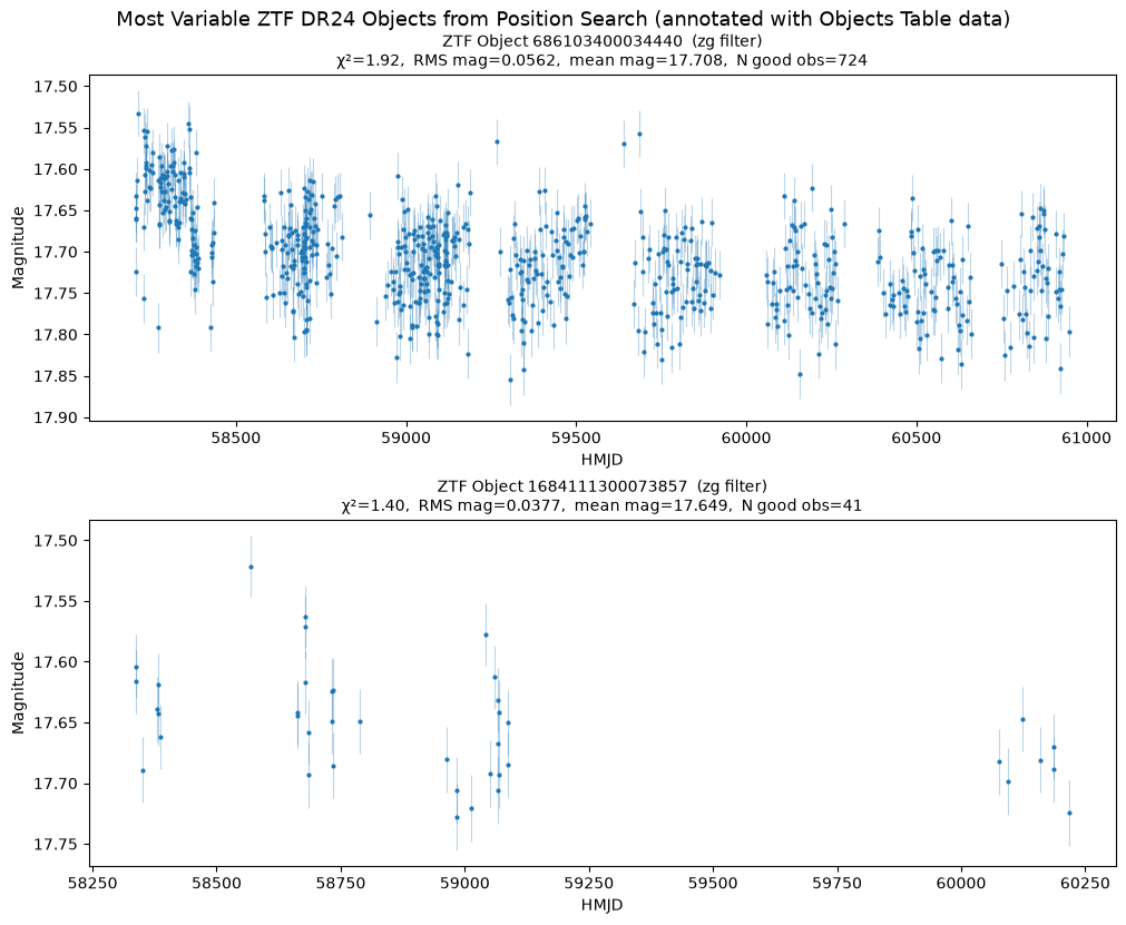

About this notebook¶

Updated: 2026-06-02

Contact: the IRSA Helpdesk with questions or to report problems.

AI Acknowledgement: This tutorial was developed with the assistance of AI tools.