Run Moving Object Search Tool (MOST) Queries

Learning Goals¶

By the end of this tutorial, you will be able to:

Run a MOST query from Python.
Identify and retrieve images intersecting the path of a moving object.
Create cutouts, centered on a moving object, from remote images on-the-fly.
Make quick co-adds of the single exposures, centered on the moving object.

Introduction¶

The Moving Object Search Tool (MOST) at NASA/IPAC Infrared Science Archive (IRSA) allows users to search for images stored at IRSA that intersect (both in time and position) the path of a moving object. Well-known objects can be searched for using their name or NAIF (Navigation and Ancillary Information Facility) ID. It is also possible to search by manually entering orbital information or using the object’s entry in the Minor Planets Center (MPC) orbit database. The astroquery module most provides a means to run these queries directly from Python. The focus of this notebook will be to describe how to run these queries and interact with their output.

MOST queries search all (NEO)WISE images by default, and this is what we will focus on below. However, it can also be used to search SPHEREx, SOFIA 2MASS, PTF, ZTF, or Spitzer, and the format of the tables returned is slightly different in each case. The orbital parameters provided in the query (either directly or by the target’s designation) are used to compute the target’s orbital path over the duration specified, and intersecting images are identified. Metadata tables containing the location of the target as a function of time and the access URLs of any intersecting images are returned by the query, and these can be used to retrieve the images and locate the target object as shown below.

Imports¶

# Uncomment the next line to install dependencies if needed.
# !pip install aiohttp 'astropy>=7.2.0' 'astroquery>=0.4.10' matplotlib numpy regions reproject requests

# For array math, deep copying, and plotting
import numpy as np
import copy
import matplotlib.pyplot as plt
from matplotlib.patches import Polygon

# Main function for running a MOST query
from astroquery.ipac.irsa.most import Most

# Key astroquery module for accessing other IRSA services
from astroquery.ipac.irsa import Irsa

# Tools for opening FITS files, making cutout, and displaying images
import astropy.io.fits as fits
from astropy.nddata import Cutout2D
from astropy.utils.data import conf
from astropy.visualization import ImageNormalize, ZScaleInterval

# For handling physical units and positions on the sky
import astropy.units as u
from astropy.coordinates import SkyCoord
from astropy.wcs import WCS

# Package for working with DS9 region files
from regions import Regions
from regions import PixCoord, PolygonSkyRegion

# Package for reprojecting images
from reproject import reproject_interp

# Astropy's default timeout limit can be too short in some cases. Increase it to 2 minutes.
conf.remote_timeout = 120

Most.clear_cache()

1. Running a MOST query and understanding the output¶

To run the MOST query we will use the query_object function from astroquery’s Most module. When querying a well-known asteroid or comet, a MOST search can usually be run with simply its name and a time window.

In all the examples in this notebook we use the (default) output mode as "Regular". We note that although "Full" is an output option, the additional output is not returned by astroquery, so the only meaningful difference will be that it takes longer to run. For more details on output modes, see the query_object docs page or the MOST instructions page.

1.1 Running the query¶

In our first example we will search for observations intersecting the path of the asteroid 128 Nemesis between December 1st 2018 and March 1st 2019.

most_output = Most.query_object(output_mode="Regular",obj_name="Nemesis",
                                obs_begin="2018-12-01",obs_end="2019-03-01")

1.2 Inspecting the output¶

The results of the query are returned in a dictionary with three keys. These keys can be displayed as follows:

most_output.keys()

dict_keys(['results', 'metadata', 'region'])

Let’s inspect each of these in turn.

First, the 'results' object is an astropy Table that lists basic information about all of the images intersecting the path of the moving object, as well are basic information about the object itself. In particular, the 'image_url' column contains the URLs at which the images can be accessed, while the 'ra_obj' and 'dec_obj' columns give the sky position of the moving object when the exposures were taken. We will make use of both of these columns below.

most_output['results']

Next, the 'metadata' object is another astropy Table that lists more information about the exposures, including the four corners of each image. If the MOST query was run in "Brief", rather than "Regular", mode then this table would be the only output.

most_output['metadata']

Finally, the 'region' object is just a string giving the URL of a DS9 regions file that contains the path of the moving object during the time window specified in the MOST query.

most_output['region']

'https://irsa.ipac.caltech.edu/workspace/TMP_X1TzIy_3008033/MOST/pid3008033/ds9region/ds9_orbit_path.reg'

2. Plotting the path of the object¶

Using the information in the DS9 regions files for the orbital path and FoVs of the exposures, we can plot the path of the object on the sky with the exposure FoVs overlaid.

2.1 Extracting exposure FoVs¶

Begin by using the Regions module to read the remote file stored at the URL for the orbital path (the 'region' element of the output above).

orb_path = Regions.read(most_output['region'], format='ds9')

Now convert the four corners of every exposure FoV (given in the 'metadata' table) to a region and add to a list of all the FoVs.

FoV_list = []
for row in most_output['metadata']:
    vertices = SkyCoord([row['ra1'], row['ra2'], row['ra3'], row['ra4']],
                        [row['dec1'], row['dec2'], row['dec3'], row['dec4']], unit=u.deg)
    FoV_list.append(PolygonSkyRegion(vertices=vertices))

2.2 Determining the plot dimensions and projection¶

In order to create a plot with the appropriate projection and extent we need to extract the minimum and maximum RA and Dec of the orbital path.

The cell below steps through every segment of the orbital path and extracts the RA and Dec values (after accounting for possible RA = 0 crossings). It then determines the extremes of RA and Dec, which will be used for setting the orbital path plot area below.

# Check for a zero crossing
RA_zero_cross = False
for i,segment in enumerate(orb_path):
    if abs(segment.end.ra.deg-segment.start.ra.deg) > 180:
        print("Caution: Likely RA = 0 crossing.")
        RA_zero_cross = True
        break

# If there is a zero crossing then switch wrap to 180 deg
if RA_zero_cross:
    for i,segment in enumerate(orb_path):
        segment.start.ra.wrap_at(180*u.deg, inplace=True)
    RA_zero_cross = False

# Extract all RA and Dec values of segments
ra_list = np.zeros(len(orb_path)*2)
dec_list = np.zeros(len(orb_path)*2)
for i,segment in enumerate(orb_path):
    ra_list[2*i] = segment.start.ra.deg
    ra_list[2*i+1] = segment.end.ra.deg
    dec_list[2*i] = segment.start.dec.deg
    dec_list[2*i+1] = segment.end.dec.deg

# Find extremes of RA and Dec
ra_min = min(ra_list)
ra_max = max(ra_list)
dec_min = min(dec_list)
dec_max = max(dec_list)

Now that the RA and Dec extremes have been determined we can set up a World Coordinate System (WCS) to define the projection of the orbit plot.

# Initialize 2D WCS
plot_wcs = WCS(naxis=2)
plot_wcs.wcs.crpix = [0,0]
plot_wcs.wcs.ctype = ["RA---SIN", "DEC--SIN"]

# Set pixel size as 1 arcmin
plot_wcs.wcs.cdelt = [-1./60., 1/60.]

# Determine the position of plot center (midway between extremes)
extremes = SkyCoord(ra=[ra_min,ra_max],dec=[dec_min,dec_max],unit=u.deg)
separation = extremes[0].separation(extremes[1])
pa = extremes[0].position_angle(extremes[1])
midpoint = extremes[0].directional_offset_by(pa, separation/2)

# Set coordinates of WCS center
plot_wcs.wcs.crval = [midpoint.ra.deg,midpoint.dec.deg]

2.3 Producing the plot¶

Finally, we can make the plot. The cell below plots the orbital path, after first ensuring the plot area is large enough to include the full path over the period in the query. It then overplots in red the fields of view of all of the exposures that intersect the path.

# Determine the range of RA and Dec values
# in order to set the number of pixel on each axis
ra_sep = separation.deg*abs(np.sin(pa))
dec_sep = separation.deg*abs(np.cos(pa))
x_npix = max(60,abs(ra_sep/plot_wcs.wcs.cdelt[0]))
y_npix = max(60,abs(dec_sep/plot_wcs.wcs.cdelt[1]))

# Don't allow aspect ratio to exceed 2:1
if not 1/2 < x_npix/y_npix < 2:
    if x_npix > y_npix:
        y_npix = x_npix/2
    else:
        x_npix = y_npix/2

# Initialize the figure, setting its dimensions
if x_npix > y_npix:
    fig = plt.figure(figsize=(8,8*y_npix/x_npix))
else:
    fig = plt.figure(figsize=(8*x_npix/y_npix,8))

# Set the axis projection with the WCS
ax = fig.add_subplot(projection=plot_wcs)

# Plot each segment of the orbital path
for segment in orb_path:
    pixel_segment = segment.to_pixel(plot_wcs)
    pixel_segment.plot(ax=ax, color='k', lw=1, ls='-')

# Overlay the exposure FoVs
for FoV in FoV_list:
    pixel_region = FoV.to_pixel(plot_wcs)
    pixel_region.plot(ax=ax, color='red', lw=1, ls='-')

# Set the limits of the x and y axes with a little padding
ax.set_xlim(np.array([-0.5,0.5])*x_npix + 0.2*min(x_npix,y_npix)*np.array([-1,1]))
ax.set_ylim(np.array([-0.5,0.5])*y_npix + 0.2*min(x_npix,y_npix)*np.array([-1,1]))
ax.set_aspect('equal')

# Set axes labels
ax.set_xlabel('RA')
ax.set_ylabel('Dec')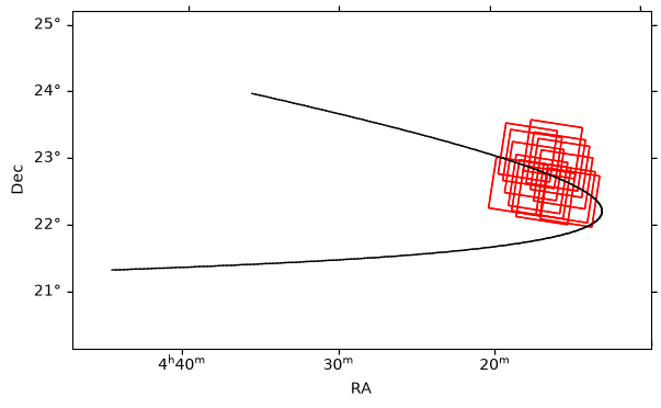

You can also generate equivalent plots using Firefly, either by submitting a solar system object query interactively on the WISE image search tool, or by launching a Firefly session from Python (as demonstrated here).

2.4 Collecting the steps into a useful function¶

We will want to produce equivalent plots later for other queries, so it makes sense to package the steps above into a plotting function that just requires the query output as its input.

def plot_path(most_output):
    '''
    Function to plot the path of a moving object
    with the FoVs of intersecting exposures overlaid.

    Parameters
    ----------
    most_output: dictionary
        The "Regular" mode output of a MOST query from
        astroquery.ipac.irsa.most.Most.query_object.
    '''

    orb_path = Regions.read(most_output['region'], format='ds9')

    FoV_list = []
    for row in most_output['metadata']:
        vertices = SkyCoord([row['ra1'], row['ra2'], row['ra3'], row['ra4']],
                            [row['dec1'], row['dec2'], row['dec3'], row['dec4']], unit=u.deg)
        FoV_list.append(PolygonSkyRegion(vertices=vertices))

    # Check for a zero crossing
    RA_zero_cross = False
    for i,segment in enumerate(orb_path):
        if abs(segment.end.ra.deg-segment.start.ra.deg) > 180:
            print("Caution: Likely RA = 0 crossing.")
            RA_zero_cross = True
            break

    # If there is a zero crossing then switch wrap to 180 deg
    if RA_zero_cross:
        for i,segment in enumerate(orb_path):
            segment.start.ra.wrap_at(180*u.deg, inplace=True)
        RA_zero_cross = False

    # Extract all RA and Dec values of segments
    ra_list = np.zeros(len(orb_path)*2)
    dec_list = np.zeros(len(orb_path)*2)
    for i,segment in enumerate(orb_path):
        ra_list[2*i] = segment.start.ra.deg
        ra_list[2*i+1] = segment.end.ra.deg
        dec_list[2*i] = segment.start.dec.deg
        dec_list[2*i+1] = segment.end.dec.deg

    # Find extremes of RA and Dec
    ra_min = min(ra_list)
    ra_max = max(ra_list)
    dec_min = min(dec_list)
    dec_max = max(dec_list)


    # Initialize 2D WCS
    plot_wcs = WCS(naxis=2)
    plot_wcs.wcs.crpix = [0,0]
    plot_wcs.wcs.ctype = ["RA---SIN", "DEC--SIN"]

    # Set pixel size as 1 arcmin
    plot_wcs.wcs.cdelt = [-1./60., 1/60.]

    # Determine the position of plot center (midway between extremes)
    extremes = SkyCoord(ra=[ra_min,ra_max],dec=[dec_min,dec_max],unit=u.deg)
    separation = extremes[0].separation(extremes[1])
    pa = extremes[0].position_angle(extremes[1])
    midpoint = extremes[0].directional_offset_by(pa, separation/2)

    # Set coordinates of WCS center
    plot_wcs.wcs.crval = [midpoint.ra.deg,midpoint.dec.deg]


    # Determine the range of RA and Dec values
    # in order to set the number of pixel on each axis
    ra_sep = separation.deg*abs(np.sin(pa))
    dec_sep = separation.deg*abs(np.cos(pa))
    x_npix = max(60,abs(ra_sep/plot_wcs.wcs.cdelt[0]))
    y_npix = max(60,abs(dec_sep/plot_wcs.wcs.cdelt[1]))

    # Don't allow aspect ratio to exceed 2:1
    if not 1/2 < x_npix/y_npix < 2:
        if x_npix > y_npix:
            y_npix = x_npix/2
        else:
            x_npix = y_npix/2

    # Initialize the figure, setting its dimensions
    if x_npix > y_npix:
        fig = plt.figure(figsize=(8,8*y_npix/x_npix))
    else:
        fig = plt.figure(figsize=(8*x_npix/y_npix,8))

    # Set the axis projection with the WCS
    ax = fig.add_subplot(projection=plot_wcs)

    # Plot each segment of the orbital path
    for segment in orb_path:
        pixel_segment = segment.to_pixel(plot_wcs)
        pixel_segment.plot(ax=ax, color='k', lw=1, ls='-')

    # Overlay the exposure FoVs
    for FoV in FoV_list:
        pixel_region = FoV.to_pixel(plot_wcs)
        pixel_region.plot(ax=ax, color='red', lw=1, ls='-')

    # Set the limits of the x and y axes with a little padding
    ax.set_xlim(np.array([-0.5,0.5])*x_npix + 0.2*min(x_npix,y_npix)*np.array([-1,1]))
    ax.set_ylim(np.array([-0.5,0.5])*y_npix + 0.2*min(x_npix,y_npix)*np.array([-1,1]))
    ax.set_aspect('equal')

    # Set axes labels
    ax.set_xlabel('RA')
    ax.set_ylabel('Dec')

    # Show plot
    plt.show()

2.5 Plotting orbital path over a very wide field¶

If, for example, you enter a date range than spans many months or even years, then the plotting method above (which uses a local sine projection) will likely fail and return a nonsensical plot. In these cases you can instead use a Mollweide projection to plot the entire sky.

For example, if we greatly expand the date range on the original query:

most_long_output = Most.query_object(output_mode="Regular",obj_name="Nemesis",
                                     obs_begin="2014-01-01",obs_end="2019-03-01")

# Extract the orbital path from the query results
long_orb_path = Regions.read(most_long_output['region'], format='ds9')

# Extract the FoVs of the overlapping images
FoV_list = []
for row in most_long_output['metadata']:
    vertices = SkyCoord([row['ra1'], row['ra2'], row['ra3'], row['ra4']],
                        [row['dec1'], row['dec2'], row['dec3'], row['dec4']], unit=u.deg)
    FoV_list.append(PolygonSkyRegion(vertices=vertices))

# Set up the figure and projection
fig = plt.figure(figsize=(8, 6))
ax = fig.add_subplot(111, projection="mollweide")

# Manually set/label the RA values
ax.set_xticklabels(["10h", "8h", "6h", "4h", "2h", "0h", "22h", "20h", "18h", "16h", "14h"])

# Overlay a coordinate grid
ax.grid(True,alpha=0.5)

# Plot each segment of the orbital path
for segment in long_orb_path:
    # Exclude any segments that would cross the entire projection
    if (segment.start.ra.wrap_at(360 * u.deg).deg < 180 and segment.end.ra.wrap_at(360 * u.deg).deg >= 180):
        pass
    elif (segment.start.ra.wrap_at(360 * u.deg).deg >= 180 and segment.end.ra.wrap_at(360 * u.deg).deg < 180):
        pass
    else:
        # The RA values need to be made negative such that they plot correctly
        ax.plot([-segment.start.ra.wrap_at(180 * u.deg).radian,-segment.end.ra.wrap_at(180 * u.deg).radian],
                [segment.start.dec.radian,segment.end.dec.radian], color='k', lw=1, ls='-', zorder=1)

# Overlay the exposure FoVs
for FoV in FoV_list:
    FoV_patch = Polygon(list(zip(-FoV.vertices.ra.radian,FoV.vertices.dec.radian)),
                        closed=True, facecolor=None, edgecolor='r',zorder=2)
    ax.add_patch(FoV_patch)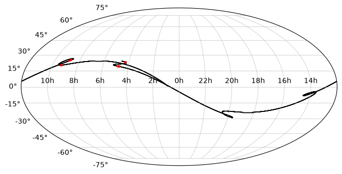

3. Displaying an image and identifying the moving object¶

We see above that the exposures listed in the results table do indeed intersect with the orbital path of Nemesis. As this is a fairly large and nearby asteroid, it should be visible in the single NEOWISE exposures identified.

3.1 Displaying a full image¶

Images can be retrieved interactively by using the solar system object tab of the mission GUIs from WISE, ZTF, and Spitzer. However, if you wish to do this in a script or notebook, then these can also be accessed programmatically.

Start by taking the URL of the first image listed in the results table.

img_access_url = most_output['results']['image_url'][0]
print(img_access_url)

https://irsa.ipac.caltech.edu/ibe/data/wise/merge/merge_p1bm_frm/9r/02659r/140/02659r140-w1-int-1b.fits

Even though the FITS file is located on a remote server it can be opened with the astropy fits package exactly as if it were a local file by passing the URL in place of the local file path.

# Open FITS file
hdul = fits.open(img_access_url)

# Extract header
header = hdul[0].header

# Extract image data
image = hdul[0].data

# Construct WCS from header
img_wcs = WCS(header)

WARNING: FITSFixedWarning: RADECSYS= 'FK5 ' 
the RADECSYS keyword is deprecated, use RADESYSa. [astropy.wcs.wcs]

We will also want to locate the target object on the image, so we should extract its position from the same row of the table.

ra_obj = most_output['results']['ra_obj'][0]*u.deg
dec_obj = most_output['results']['dec_obj'][0]*u.deg

# Create SkyCoord object of object position
pos_obj = SkyCoord(ra=ra_obj, dec=dec_obj)

# Convert to pixel location via the WCS
pix_pos_obj = pos_obj.to_pixel(img_wcs)

Now display the image and point to the object.

# Initialize figure
fig = plt.figure(figsize=(8,8))
ax = fig.add_subplot(projection=img_wcs)

# Use the ZScale interval (similar to DS9) to normalize the intensity
norm = ImageNormalize(image, interval=ZScaleInterval())

# Display the figure
ax.imshow(image,origin='lower',norm=norm,cmap='Greys_r')

# Add orange arrow pointing to object
ax.annotate('',pix_pos_obj-0.01*np.array([header['NAXIS1'],header['NAXIS2']]),
            pix_pos_obj-0.1*np.array([header['NAXIS1'],header['NAXIS2']]),
            arrowprops={'width':2, 'facecolor':'orange', 'edgecolor':'none'})

# Label axes and overlay coordinate grid
ax.set_xlabel('RA')
ax.set_ylabel('Dec')
ax.coords.grid(color='lime', linestyle='solid', alpha=0.3)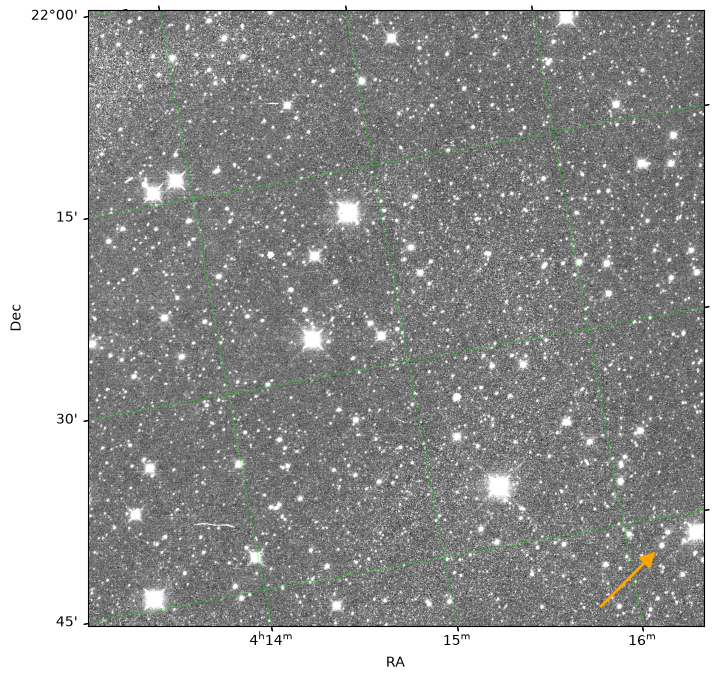

There does appear to be a bright object indicated by the arrow, but really we need to know if this moves as expected from image to image, as time progresses and the target object moves along its orbital path.

3.2 Making cutouts and comparing to the AllWISE Atlas¶

We could display the full image for every exposure listed in the results table, however, this would involve downloading a lot of data when really we’re only interested in a small region immediately around where we expect to find the target object. Below we will use the astropy Cutout2D function to extract cutouts from the remote images without downloading the full FITS file. This will allow us to see the portions of the images that are most relevant, while saving a lot of bandwidth (and speeding up the execution).

To start we will order the 'metadata' table by observation date (MJD) and then by band, so that images appear in the order they were observed and with shorter wavelength images appearing first. This adds some complications to the following code, but will aid the interpretation of the cutouts. In particular, as we are re-ordering one of the tables, we must now use the 'image_ID' column in the 'results' table to relate the rows in the 'metadata' table to those in the 'results' table.

# Duplicate metadata table
ordered_metadata = most_output['metadata']

# Sort by date then band
ordered_metadata.sort(['mjd_obs','band'])

# Construct the image IDs to relate rows to those in the results table
imgIDs = []
for i in range(len(ordered_metadata)):
    imgIDs.append(f"{ordered_metadata[i]['scan_id']}_{ordered_metadata[i]['frame_num']}_{ordered_metadata[i]['band']}")
ordered_metadata['Image_ID'] = imgIDs

# Duplicate results table and index by image ID
indexed_results = most_output['results']
indexed_results.add_index('Image_ID')

Below (collapsed cell) we create two functions for producing cutouts of remotely hosted FITS images. The first creates a cutout of a single image, given the URL to access the image at, the center of the intended cutout, and its size. The second function is similar, except that it will automatically identify the AllWISE image at a given location, by submitting a Simple Image Access (SIA) v2 query to IRSA’s SIAv2 service using the astroquery function query_sia, and use this image to produce the cutout. In addition, the second function takes a cutout (generated by the first function) as input, so that it can reproject to exactly match the orientation, as well as the center wavelength of the WISE band to generate the cutout from.

def exposure_cutout(image_url,cutout_center,cutout_size):
    '''
    Function to make FITS image cutout.

    Parameters
    ----------
    image_url: string
        URL (or path) of the FITS file to make
        cutout from.
    cutout_center: SkyCoord object
        Position of the cutout's center.
    cutout_size: astropy Quantity
        Cutout size (square) in angular units.

    Outputs
    -------
    cutout: Cutout2D object
        Image cutout, including data, WCS, and shape.
    norm: ImageNormalize object
        Normalization of cutout data for plotting
        with matplotlib.
    header: FITS Header object
        FITS header of the parent image.
    '''

    # Open remote FITS file and extract cutout
    with fits.open(image_url, use_fsspec=True) as hdul:
        header = hdul[0].header
        img_wcs = WCS(header)
        cutout = Cutout2D(hdul[0].section, position=cutout_center,
                          size=cutout_size.to(u.arcsec).value/abs(header['PXSCAL2']),
                          wcs=img_wcs,mode='partial', fill_value=np.nan)

    # Normalize cutout intensity
    norm = ImageNormalize(cutout.data, interval=ZScaleInterval())

    return cutout, norm, header


def reference_cutout(cutout_center,cutout,cutout_size,centwave):
    '''
    Function to make FITS image cutout from AllWISE
    at specified location, and match projection of
    an existing cutout.

    Parameters
    ----------
    cutout_center: SkyCoord object
        Position of the cutout's center.
    cutout: Cutout2D object
        Existing cuout for matching projection.
    cutout_size: astropy Quantity
        Cutout size (square) in angular units.
    centwave: float
        The center wavelength of the WISE band
        to make the cutout from (in m).

    Outputs
    -------
    ref_cutout: Cutout2D object
        Image cutout, including data, WCS, and shape.
    norm: ImageNormalize object
        Normalization of cutout data for plotting
        with matplotlib.
    header: FITS Header object
        FITS header of the parent image.
    '''

    # Query the IRSA SIAv2 service for the AllWISE image at this position
    allwise_img_tab = Irsa.query_sia(pos=(cutout_center, 1 * u.arcmin),
                                     collection='wise_allwise', band=centwave)

    # Get access URL from the query results
    allwise_img_url = allwise_img_tab[allwise_img_tab['dataproduct_subtype'] == 'science'][0]['access_url']

    # Open the image and extract a cutout
    # Extract a larger cutout than above as it will need to be reprojected
    with fits.open(allwise_img_url, use_fsspec=True) as hdul:
        header = hdul[0].header
        img_wcs = WCS(header)
        ref_cutout = Cutout2D(hdul[0].section, position=cutout_center,size=2*cutout_size,wcs=img_wcs,
                              mode='partial', fill_value=np.nan)

    # Use the reproject function to project the reference cutout
    # to the same WCS as the target cutout
    ref_cutout, footprint = reproject_interp(input_data=(ref_cutout.data, ref_cutout.wcs),
                                             output_projection=cutout.wcs,
                                             shape_out=cutout.shape)

    # Normalize the intensity and display
    norm = ImageNormalize(ref_cutout.data, interval=ZScaleInterval())

    return ref_cutout, norm, header

Now we are ready to make and display the cutouts.

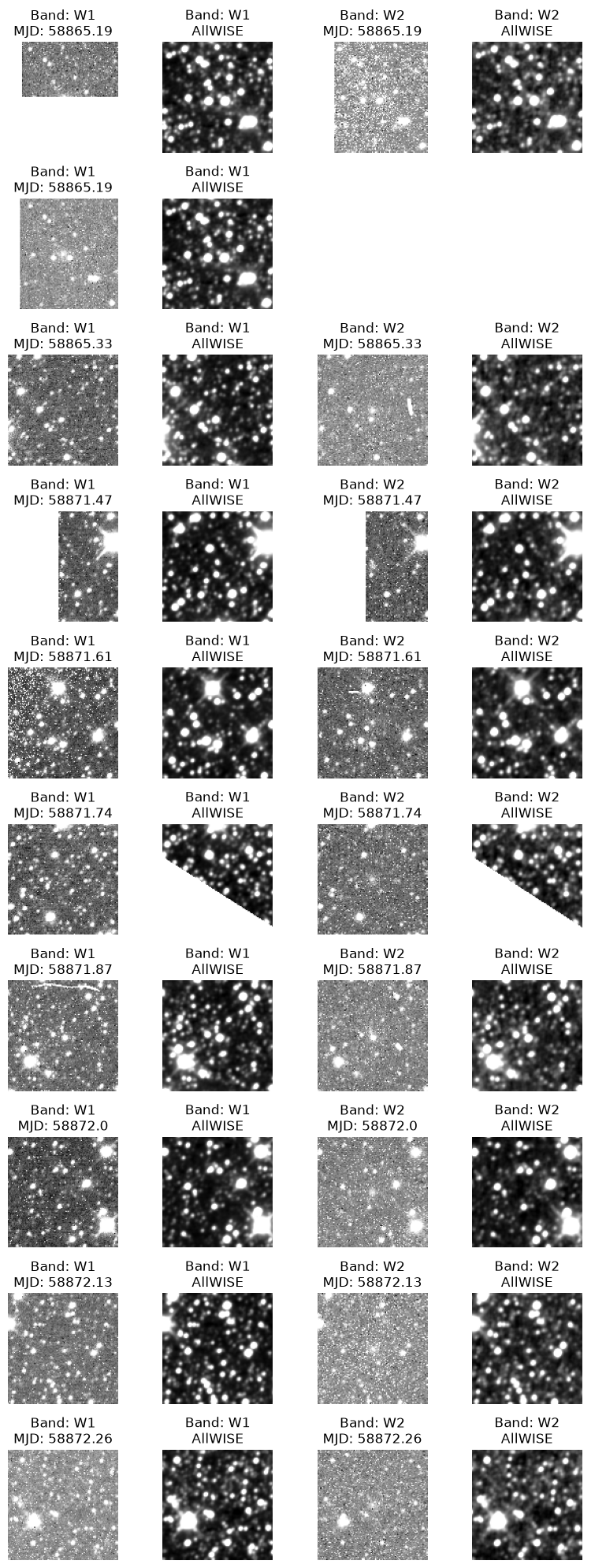
The following cell sets up a grid of subplots based on the number of exposures that were found in the query and the number of unique bands. A loop cycles through all of the blank subplots in the grid and a cutout is generated from each image listed in the 'metadata' table at the expected location of the moving object.

For every cutout of a NEOWISE exposure, a second cutout from AllWISE (in the same band) is also created, and acts as a reference for fixed background sources that do not move.

# Set number of bands (max of 4 for WISE)
n_band = min(4,len(set(ordered_metadata['band'])))
band_names = list(set(ordered_metadata['band']))
band_names.sort()

# Set the number of images (max set at 10)
n_img = min(10,len(set(ordered_metadata['scan_id'])))

# Set the WISE band center wavelengths (m)
# Used in SIAv2 query to return the correct band
wise_bands_centwave = [3.4E-6,4.6E-6,1.2E-5,2.2E-5]

# Initialize the subplot array
fig, ax_arr = plt.subplots(nrows=n_img, ncols=2*n_band,
                           figsize=2*np.array([2*n_band,n_img]))

# Hide all axes
for i in range(n_img):
    for j in range(2*n_band):
        ax = ax_arr[i][j]
        ax.set_axis_off()

# Set the cutout size
cutout_size = 5*u.arcmin


# Initialize a counter to keep track of
# the number of cutouts displayed
counter = 0

# Save the ID of the previous scan in the loop
# initialize with the first ID
prev_scanID = ordered_metadata['scan_id'][0]

# Loop over the grid
for i in range(n_img):
    for j in range(n_band):

        # Check if the current scan ID is the same as the previous
        # If not, then go to the next row of the plot grid
        scanID = ordered_metadata['scan_id'][counter]
        if (scanID not in prev_scanID) and (j != 0):
            prev_scanID = copy.deepcopy(scanID)
            break
        else:
            prev_scanID = copy.deepcopy(scanID)

        # Extract position of target object
        ra_obj = ordered_metadata['ra_obj'][counter]*u.deg
        dec_obj = ordered_metadata['dec_obj'][counter]*u.deg
        pos_obj = SkyCoord(ra=ra_obj, dec=dec_obj)

        # Set axis for displaying cutout
        ax = ax_arr[i][2*j]

        # Create single exposure cutout
        cutout, norm, header = exposure_cutout(indexed_results.loc[ordered_metadata['Image_ID'][counter]]['image_url'],
                                       pos_obj,cutout_size)

        # Display on figure
        ax.imshow(cutout.data,origin='lower',norm=norm,cmap='Greys_r')

        # Add title indicating the band and date
        ax.set_title(f"Band: W{band_names[j]}\nMJD: {np.round(header['MJD_OBS'], 2)}")


        # Now make reference cutout

        # Set axis for displaying cutout
        ax = ax_arr[i][2*j+1]

        # Create matching AllWISE reference cutout
        ref_cutout, norm, header = reference_cutout(pos_obj,cutout,cutout_size,wise_bands_centwave[j])

        # Display on figure
        ax.imshow(ref_cutout.data,origin='lower',norm=norm,cmap='Greys_r')

        # Add title indicating the band and date
        ax.set_title(f'Band: W{band_names[j]}\nAllWISE')

        # Increment counter
        counter += 1

plt.tight_layout()

WARNING: FITSFixedWarning: RADECSYS= 'FK5 ' 
the RADECSYS keyword is deprecated, use RADESYSa. [astropy.wcs.wcs]

WARNING: FITSFixedWarning: RADECSYS= 'FK5 ' 
the RADECSYS keyword is deprecated, use RADESYSa. [astropy.wcs.wcs]

WARNING: FITSFixedWarning: RADECSYS= 'FK5 ' 
the RADECSYS keyword is deprecated, use RADESYSa. [astropy.wcs.wcs]

WARNING: FITSFixedWarning: RADECSYS= 'FK5 ' 
the RADECSYS keyword is deprecated, use RADESYSa. [astropy.wcs.wcs]

WARNING: FITSFixedWarning: RADECSYS= 'FK5 ' 
the RADECSYS keyword is deprecated, use RADESYSa. [astropy.wcs.wcs]

WARNING: FITSFixedWarning: RADECSYS= 'FK5 ' 
the RADECSYS keyword is deprecated, use RADESYSa. [astropy.wcs.wcs]

WARNING: FITSFixedWarning: RADECSYS= 'FK5 ' 
the RADECSYS keyword is deprecated, use RADESYSa. [astropy.wcs.wcs]

WARNING: FITSFixedWarning: RADECSYS= 'FK5 ' 
the RADECSYS keyword is deprecated, use RADESYSa. [astropy.wcs.wcs]

WARNING: FITSFixedWarning: RADECSYS= 'FK5 ' 
the RADECSYS keyword is deprecated, use RADESYSa. [astropy.wcs.wcs]

WARNING: FITSFixedWarning: RADECSYS= 'FK5 ' 
the RADECSYS keyword is deprecated, use RADESYSa. [astropy.wcs.wcs]

WARNING: FITSFixedWarning: RADECSYS= 'FK5 ' 
the RADECSYS keyword is deprecated, use RADESYSa. [astropy.wcs.wcs]

WARNING: FITSFixedWarning: RADECSYS= 'FK5 ' 
the RADECSYS keyword is deprecated, use RADESYSa. [astropy.wcs.wcs]

WARNING: FITSFixedWarning: RADECSYS= 'FK5 ' 
the RADECSYS keyword is deprecated, use RADESYSa. [astropy.wcs.wcs]

WARNING: FITSFixedWarning: RADECSYS= 'FK5 ' 
the RADECSYS keyword is deprecated, use RADESYSa. [astropy.wcs.wcs]

WARNING: FITSFixedWarning: RADECSYS= 'FK5 ' 
the RADECSYS keyword is deprecated, use RADESYSa. [astropy.wcs.wcs]

WARNING: FITSFixedWarning: RADECSYS= 'FK5 ' 
the RADECSYS keyword is deprecated, use RADESYSa. [astropy.wcs.wcs]

WARNING: FITSFixedWarning: RADECSYS= 'FK5 ' 
the RADECSYS keyword is deprecated, use RADESYSa. [astropy.wcs.wcs]

WARNING: FITSFixedWarning: RADECSYS= 'FK5 ' 
the RADECSYS keyword is deprecated, use RADESYSa. [astropy.wcs.wcs]

WARNING: FITSFixedWarning: RADECSYS= 'FK5 ' 
the RADECSYS keyword is deprecated, use RADESYSa. [astropy.wcs.wcs]

WARNING: FITSFixedWarning: RADECSYS= 'FK5 ' 
the RADECSYS keyword is deprecated, use RADESYSa. [astropy.wcs.wcs]

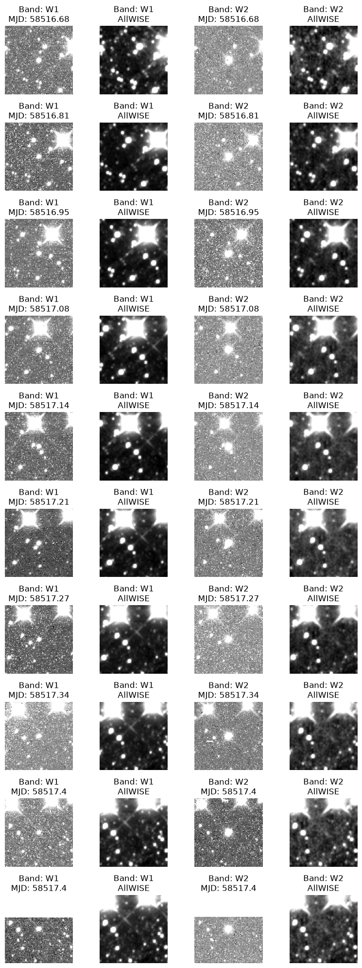
The asteroid is clearly visible as a bright point source at the center of each of the single exposure cutouts, but is absent from the AllWISE reference cutouts. Furthermore, the source moves from frame to frame, relative to the background sources, confirming that it is a moving object and the cutouts are correctly centered. That it always falls in the center of the cutout indicates that its orbital parameters are well-known and its position can be predicted accurately. In less clear cut cases it may be useful to also explore the AllWISE source catalog along with the cutouts. This can be done interactively by submitting a solar system object query in the IRSA WISE interface.

We will also need to generate equivalent cutouts again below, so once again we can collect the cells above into a single function that will retrieve and plot the cutouts.

def plot_cutouts(most_output, return_stack=False):
    '''
    Function to plot (NEO)WISE cutouts identifed in a
    MOST query_object query. Up to a maximum of 10 cutouts
    in each band. Reference AllWISE cutouts are also plotted.

    Parameters
    ----------
    most_output: dictionary
        The "Regular" mode output of a MOST query from
        astroquery.ipac.irsa.most.Most.query_object.
    return_stack: bool (Default: False)
        Option to return the stack of cutouts.

    Outputs
    -------
    stack: list
        A list of numpy.array objects containing the pixel
        values of the cutouts (in nanomaggies). Only returned
        if return_stack parameter is True.
        The list contains lists of arrays
    '''

    # Duplicate metadata table
    ordered_metadata = most_output['metadata']

    # Sort by date then band
    ordered_metadata.sort(['mjd_obs','band'])

    # Construct the image IDs to relate rows to those in the results table
    imgIDs = []
    for i in range(len(ordered_metadata)):
        imgIDs.append(f"{ordered_metadata[i]['scan_id']}_{ordered_metadata[i]['frame_num']}_{ordered_metadata[i]['band']}")
    ordered_metadata['Image_ID'] = imgIDs

    # Duplicate results table and index by image ID
    indexed_results = most_output['results']
    indexed_results.add_index('Image_ID')


    # Set number of bands (max of 4 for WISE)
    n_band = min(4,len(set(ordered_metadata['band'])))
    band_names = list(set(ordered_metadata['band']))
    band_names.sort()

    # Set the number of images (max set at 10)
    n_img = min(10,len(set(ordered_metadata['scan_id'])))

    # Set the WISE band center wavelengths (m)
    # Used in SIAv2 query to return the correct band
    wise_bands_centwave = [3.4E-6,4.6E-6,1.2E-5,2.2E-5]

    # Initialize the subplot array
    fig, ax_arr = plt.subplots(nrows=n_img, ncols=2*n_band,
                               figsize=2*np.array([2*n_band,n_img]))

    # Hide all axes
    for i in range(n_img):
        for j in range(2*n_band):
            ax = ax_arr[i][j]
            ax.set_axis_off()

    # Set the cutout size
    cutout_size = 5*u.arcmin


    # Initialize a counter to keep track of
    # the number of cutouts displayed
    counter = 0

    # Save the ID of the previous scan in the loop
    # initialize with the first ID
    prev_scanID = ordered_metadata['scan_id'][0]

    # Loop over the grid
    for i in range(n_img):
        for j in range(n_band):

            # Check if the current scan ID is the same as the previous
            # If not, then go to the next row of the plot grid
            scanID = ordered_metadata['scan_id'][counter]
            if (scanID not in prev_scanID) and (j != 0):
                prev_scanID = copy.deepcopy(scanID)
                break
            else:
                prev_scanID = copy.deepcopy(scanID)

            # Extract position of target object
            ra_obj = ordered_metadata['ra_obj'][counter]*u.deg
            dec_obj = ordered_metadata['dec_obj'][counter]*u.deg
            pos_obj = SkyCoord(ra=ra_obj, dec=dec_obj)

            # Set axis for displaying cutout
            ax = ax_arr[i][2*j]

            # Create single exposure cutout
            cutout, norm, header = exposure_cutout(indexed_results.loc[ordered_metadata['Image_ID'][counter]]['image_url'],
                                                   pos_obj,cutout_size)

            # Display on figure
            ax.imshow(cutout.data,origin='lower',norm=norm,cmap='Greys_r')

            # Add title indicating the band and date
            ax.set_title(f"Band: W{band_names[j]}\nMJD: {np.round(header['MJD_OBS'], 2)}")

            # Check if stack already exists
            if 'stack' not in locals():
                stack = np.zeros(shape=(2*n_band,n_img,cutout.shape[0],cutout.shape[1])) + np.nan

            # Place cutout in stack
            stack[2*j][i] = np.array(cutout.data)


            # Now make reference cutout

            # Set axis for displaying cutout
            ax = ax_arr[i][2*j+1]

            # Create matching AllWISE reference cutout
            ref_cutout, norm, header = reference_cutout(pos_obj,cutout,cutout_size,wise_bands_centwave[j])

            # Display on figure
            ax.imshow(ref_cutout.data,origin='lower',norm=norm,cmap='Greys_r')

            # Add title indicating the band and date
            ax.set_title(f'Band: W{band_names[j]}\nAllWISE')

            # Place reference cutout in stack
            stack[2*j+1][i] = np.array(ref_cutout.data)

            # Increment counter
            counter += 1

    plt.tight_layout()

    if return_stack:
        return stack

4. Stacking cutouts to aid detection¶

In many cases the moving object searched for will not be visible in a single exposure. In these cases it can be useful to stack the exposures to gain sensitivity.

4.1 A new object and a manual input query¶

In this example we will look for NEOWISE imaging intersecting with the path of 2I/Borisov, the second ever confirmed extrasolar object to be identified passing through the solar system.

most_output = Most.query_object(output_mode="Regular",obj_name="2I",
                                obs_begin="2020-01-01",obs_end="2020-02-01")

Use the function that we defined above to plot the orbit.

plot_path(most_output)

4.2 Plot and stack cutouts¶

Now we can use the other function defined above to plot the first 10 cutouts in each band.

An additional feature that was added in the function definition, but not shown in the example above, is the option to return a stack containing all of the cutouts. We will do this here as they will be needed below.

stack = plot_cutouts(most_output,return_stack=True)

WARNING: FITSFixedWarning: RADECSYS= 'FK5 ' 
the RADECSYS keyword is deprecated, use RADESYSa. [astropy.wcs.wcs]

WARNING: FITSFixedWarning: RADECSYS= 'FK5 ' 
the RADECSYS keyword is deprecated, use RADESYSa. [astropy.wcs.wcs]

WARNING: FITSFixedWarning: RADECSYS= 'FK5 ' 
the RADECSYS keyword is deprecated, use RADESYSa. [astropy.wcs.wcs]

WARNING: FITSFixedWarning: RADECSYS= 'FK5 ' 
the RADECSYS keyword is deprecated, use RADESYSa. [astropy.wcs.wcs]

WARNING: FITSFixedWarning: RADECSYS= 'FK5 ' 
the RADECSYS keyword is deprecated, use RADESYSa. [astropy.wcs.wcs]

WARNING: FITSFixedWarning: RADECSYS= 'FK5 ' 
the RADECSYS keyword is deprecated, use RADESYSa. [astropy.wcs.wcs]

WARNING: FITSFixedWarning: RADECSYS= 'FK5 ' 
the RADECSYS keyword is deprecated, use RADESYSa. [astropy.wcs.wcs]

WARNING: FITSFixedWarning: RADECSYS= 'FK5 ' 
the RADECSYS keyword is deprecated, use RADESYSa. [astropy.wcs.wcs]

WARNING: FITSFixedWarning: RADECSYS= 'FK5 ' 
the RADECSYS keyword is deprecated, use RADESYSa. [astropy.wcs.wcs]

WARNING: FITSFixedWarning: RADECSYS= 'FK5 ' 
the RADECSYS keyword is deprecated, use RADESYSa. [astropy.wcs.wcs]

WARNING: FITSFixedWarning: RADECSYS= 'FK5 ' 
the RADECSYS keyword is deprecated, use RADESYSa. [astropy.wcs.wcs]

WARNING: FITSFixedWarning: RADECSYS= 'FK5 ' 
the RADECSYS keyword is deprecated, use RADESYSa. [astropy.wcs.wcs]

WARNING: FITSFixedWarning: RADECSYS= 'FK5 ' 
the RADECSYS keyword is deprecated, use RADESYSa. [astropy.wcs.wcs]

WARNING: FITSFixedWarning: RADECSYS= 'FK5 ' 
the RADECSYS keyword is deprecated, use RADESYSa. [astropy.wcs.wcs]

WARNING: FITSFixedWarning: RADECSYS= 'FK5 ' 
the RADECSYS keyword is deprecated, use RADESYSa. [astropy.wcs.wcs]

WARNING: FITSFixedWarning: RADECSYS= 'FK5 ' 
the RADECSYS keyword is deprecated, use RADESYSa. [astropy.wcs.wcs]

WARNING: FITSFixedWarning: RADECSYS= 'FK5 ' 
the RADECSYS keyword is deprecated, use RADESYSa. [astropy.wcs.wcs]

WARNING: FITSFixedWarning: RADECSYS= 'FK5 ' 
the RADECSYS keyword is deprecated, use RADESYSa. [astropy.wcs.wcs]

WARNING: FITSFixedWarning: RADECSYS= 'FK5 ' 
the RADECSYS keyword is deprecated, use RADESYSa. [astropy.wcs.wcs]

Although the eagle-eyed among us may be able to detect 2I/Borisov in some of the cutouts (primarily W2), in general, stacking the cutouts will give a better indication of how confidently the source is/isn’t detected.

The cell below median combines the single exposure cutouts to boost sensitivity.

# Set number of unique bands
n_bands = min(2,len(set(most_output['metadata']['band'])))

# initialize the figure and axes
fig, ax_arr = plt.subplots(nrows=1, ncols=n_bands,
                           figsize=2*np.array([n_bands,1]))

# Hide all axes
for j in range(n_bands):
    ax = ax_arr[j]
    ax.set_axis_off()

# Loop over all bands
for j in range(n_bands):

    # Set current axis
    ax = ax_arr[j]

    # Median combine the single exposure cutouts
    band_stack = np.nanmedian(stack[2*j],axis=0)

    # Normalize the intensity and display
    norm = ImageNormalize(band_stack, interval=ZScaleInterval())
    ax.imshow(band_stack,origin='lower',norm=norm,cmap='Greys_r')
    ax.set_title(f'W{j+1} target stack')

plt.tight_layout()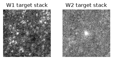

2I/Borisov is now clearly visible in the W2 cutout and marginally detected in W1 as well.

Tip

If you have already run a MOST query in Python and wish to make a stacked cutout with ICORE, the input table required can be generated with the commands:

from astropy.io import ascii
ascii.write(most_output['metadata'], output="metadata_table.tbl", format='ipac', overwrite=True)

5. SPHEREx¶

Support for SPHEREx in MOST was added in June 2026. SPHEREx images can be obtained in much the same way as the WISE examples shown above by setting the 'catalog' argument to "spherex".

Here we search for images containing the asteroid Vesta taken during August 2025.

most_output = Most.query_object(output_mode="Regular",obj_name="Vesta",
                                obs_begin="2025-08-01",obs_end="2025-08-31",
                                catalog="spherex")

The orbital path can be plotted using the same function as before.

plot_path(most_output)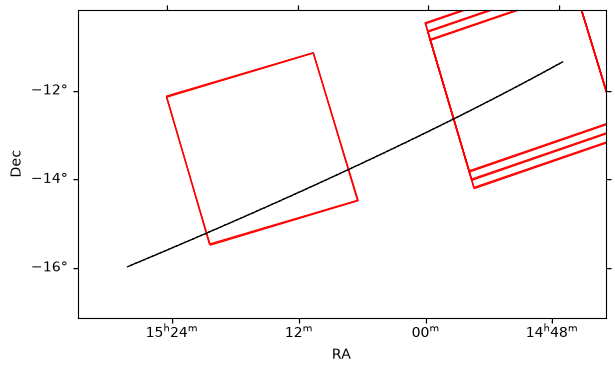

A cutout can be produced in much the same way as before, although minor changes are needed as the headers of the SPHEREx images differ from those of WISE.

# Get the URL for the first image in the MOST output
img_access_url = most_output['results']['image_url'][0]
print(img_access_url)

# Get the position of target corresponding to the first image
ra_obj = most_output['results']['ra_obj'][0]*u.deg
dec_obj = most_output['results']['dec_obj'][0]*u.deg

# Create SkyCoord object of object position
pos_obj = SkyCoord(ra=ra_obj, dec=dec_obj)

# Set cutout size
cutout_size = 5*u.arcmin

# Open remote FITS file and extract cutout
with fits.open(img_access_url, use_fsspec=True) as hdul:
    header = hdul[1].header
    pixel_scale = np.sqrt(header['PC1_1']**2 + header['PC1_2']**2)
    img_wcs = WCS(header)

    cutout = Cutout2D(hdul[1].data, position=pos_obj,
                      size=cutout_size.to(u.deg).value/pixel_scale,
                      wcs=img_wcs,mode='partial', fill_value=np.nan)

    # Normalize cutout intensity
    norm = ImageNormalize(cutout.data, interval=ZScaleInterval())

https://irsa.ipac.caltech.edu/ibe/data/spherex/qr2/level2/2025W32_1A/l2b-v20-2025-264/6/level2_2025W32_1A_0105_1D6_spx_l2b-v20-2025-264.fits

# Initialize figure
fig = plt.figure(figsize=(6,6))
ax = fig.add_subplot(projection=cutout.wcs)

# Display the figure
ax.imshow(cutout.data,origin='lower',norm=norm,cmap='Greys_r')

# Overlay coordinate grid
ax.set_xlabel('RA')
ax.set_ylabel('Dec')
ax.coords.grid(color='lime', linestyle='solid', alpha=0.3)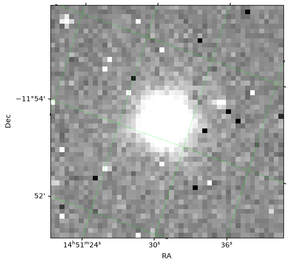

6. New discoveries: Queries using orbital elements and the MPC one-line format¶

Although in general it is strongly recommended to use object names to perform searches, in the rare case of a new discovery where the object is not yet in JPL Horizons, MOST allows the input of orbital elements or the one-line MPC format. These are most effective for times close to the epoch of the elements.

To use the one-line MPC format in a MOST query the input_type must be set to "mpc_input", and the one line entry in the MPC orbit database provided as a string.

In the example below we use the first known interstellar object in the solar system 'Oumuamua, which can be found near the bottom of the comets database file.

Oumuamua_MPC_entry = "0001I         2017 09  9.4886  0.255240  1.199252  241.6845   24.5997  122.6778  20170904  23.0  2.0  1I/`Oumuamua                                             MPC107687"

The query can now be run as follows:

most_output = Most.query_object(output_mode="Regular",input_mode="mpc_input",
                                obs_begin="2017-03-01",obs_end="2017-05-01",obj_type="Comet",
                                mpc_data=Oumuamua_MPC_entry)

The format of the output is exactly as for the previous queries and we can use the same functions to interact with it. For example:

plot_path(most_output)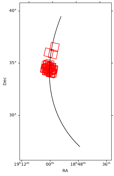

In addition to the MPC one-line format, orbital elements can also be listed manually one-by-one as arguments in the query_object function. The exact same search for 2I/Borisov performed above (Section 4) using its name, "2I", can also be performed by entering its orbital elements directly. Several epochs of orbit parameters are available for 2I/Borisov and its orbit changed significantly over time (due in part to outgassing). If we look for the one line MPCORB database entry for 2I/Borisov, it will list only the paramters for the latest epoch. However, these will not be appropriate for locating it in January 2020, which is when we wish to search for intersecting images.

To find the orbital parameters for prior epochs, search for “2I” on the MPC Database Search page. In this case the epoch including Jan. 2020 is 2019-12-23.0, and we will use the parameters from this epoch in our query below. The orbital parameters listed can then be entered into the query_object function with the input_type set as "manual_input" and obj_type as "Comet", as follows:

most_output = Most.query_object(output_mode="Regular",input_mode="manual_input",
                                obs_begin="2020-01-01",obs_end="2020-02-01",obj_type="Comet",
                                epoch=58840.0,eccentricity=3.3565579,inclination=44.05262,
                                arg_perihelion=209.12389,ascend_node=308.14778,
                                perih_dist=2.0065337,perih_time=2458826.05305)

plot_path(most_output)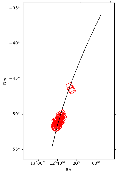

Acknowledgements¶

Caltech/IPAC-IRSA

About this notebook¶

Authors: Michael G. Jones, Brigitta Sipőcz, and Tim Brooke

Updated: 25 June 2026

Contact: IRSA Helpdesk with questions or problems.

Runtime: As of the date above, this notebook takes about 10 minutes to run to completion on a machine with 32GB RAM and 12 CPUs. However, the notebook is heavily dependent on archive servers which means runtime will likely vary significantly from user to user.