Download a collection of SPHEREx Spectral Image cutouts as a multi-extension FITS file
1. Learning Goals
Perform a query for the list of SPHEREx Spectral Image Multi-Extension FITS files (MEFs) that overlap a given coordinate.
Retrieve cutouts for every entry in this list and package the cutouts as a new MEF.
Learn how to use parallel or serial processing to retrieve the cutouts.
2. SPHEREx Overview
SPHEREx is a NASA Astrophysics Medium Explorer mission that launched in March 2025. During its planned two-year mission, SPHEREx will obtain 0.75-5 micron spectroscopy over the entire sky, with deeper data in the SPHEREx Deep Fields. SPHEREx data will be used to:
constrain the physics of inflation by measuring its imprints on the three-dimensional large-scale distribution of matter,
trace the history of galactic light production through a deep multi-band measurement of large-scale clustering,
investigate the abundance and composition of water and biogenic ices in the early phases of star and planetary disk formation.
The community will also mine SPHEREx data and combine it with synergistic data sets to address a variety of additional topics in astrophysics.
More information is available in the SPHEREx Explanatory Supplement.
3. Imports
The following packages must be installed to run this notebook.
# Uncomment the next line to install dependencies if needed.
# !pip install numpy astropy pyvo matplotlib
import concurrent.futures
import http.client
import time
import urllib.error
import astropy.units as u
import matplotlib.pyplot as plt
import numpy as np
import pyvo
from astropy.coordinates import SkyCoord
from astropy.io import fits
from astropy.table import Table
from astropy.wcs import WCS
# Suppress logging temporarily to prevent astropy
# from repeatedly printing out warning notices related to alternate WCSs
import logging
logging.getLogger('astropy').setLevel(logging.ERROR)
# The time it takes to read SPHEREx files can exceed
# astropy's default timeout limit. Increase it.
from astropy.utils.data import conf
conf.remote_timeout = 1204. Specify inputs and outputs
Specify a right ascension, declination, cutout size, and a SPHEREx bandpass (e.g., ‘SPHEREx-D2’).
In this example, we are creating cutouts of the Pinwheel galaxy (M101) for the SPHEREx detector D2.
# Choose a position.
ra = 210.80227 * u.degree
dec = 54.34895 * u.degree

# Choose a cutout size.
size = 0.1 * u.degree

# Choose the bandpass of interest.
bandpass = 'SPHEREx-D2'

# Choose an output filename root for the output MEF file.
output_filename = 'spherex_cutouts_mef.fits'
5. Query IRSA for a list of cutouts that satisfy the criteria specified above.
Here we show how to use the pyvo TAP SQL query to retrieve all images that overlap with the position defined above.
This query will retrieve a table of URLs that link to the MEF cutouts.
Each row in the table corresponds to a single cutout and includes the data access URL and an observation timestamp.
The results are sorted from oldest to newest.
# Define the service endpoint for IRSA's Table Access Protocol (TAP)
# so that we can query SPHEREx metadata tables.
service = pyvo.dal.TAPService("https://irsa.ipac.caltech.edu/TAP")

# Define a query that will search the appropriate SPHEREx metadata tables
# for spectral images that cover the chosen coordinates and match the
# specified bandpass. Return the cutout data access URL and the time of observation.
# Sort by observation time.
query = f"""
SELECT
    'https://irsa.ipac.caltech.edu/' || a.uri || '?center={ra.value},{dec.value}d&size={size.value}' AS uri,
    p.time_bounds_lower
FROM spherex.artifact a
JOIN spherex.plane p ON a.planeid = p.planeid
WHERE 1 = CONTAINS(POINT('ICRS', {ra.value}, {dec.value}), p.poly)
        AND p.energy_bandpassname = '{bandpass}'
ORDER BY p.time_bounds_lower
"""

# Execute the query and return as an astropy Table.
t1 = time.time()
results = service.search(query)
print("Time to do TAP query: {:2.2f} seconds.".format(time.time() - t1))
print("Number of images found: {}".format(len(results)))
Time to do TAP query: 8.68 seconds.
Number of images found: 52
6. Define a function that processes a list of SPHEREx Spectral Image Cutouts
This function takes in a row of the catalog that we created above and does the following:
It downloads the cutout
It computes the wavelength of the center pixel of the cutout (in micro-meters)
It combines the image HDUs into a new HDU and adds it to the table row.
Note that the values of the rows are being added in place.
def process_cutout(row, ra, dec, cache):
    '''
    Downloads the cutouts given in a row of the table including all SPHEREx images overlapping with a position.

    Parameters:
    ===========

    row : astropy.table row
        Row of a table that will be changed in place by this function. The table
        is created by the SQL TAP query.
    ra,dec : coordinates (astropy units)
        Ra and Dec coordinates (same as used for the TAP query) with attached astropy units
    cache : bool
        If set to `True`, the output of cached and the cutout processing will run faster next time.
        Turn this feature off by setting `cache = False`.
    '''

    with fits.open(row["uri"], cache=cache) as hdulist:
        # There are seven HDUs:
        # 0 contains minimal metadata in the header and no data.
        # 1 through 6 are: IMAGE, FLAGS, VARIANCE, ZODI, PSF, WCS-WAVE
        header = hdulist[1].header

        # Compute pixel coordinates corresponding to cutout position.
        spatial_wcs = WCS(header)
        x, y = spatial_wcs.world_to_pixel(SkyCoord(ra=ra, dec=dec, unit="deg", frame="icrs"))

        # Compute wavelength at cutout position.
        spectral_wcs = WCS(header, fobj=hdulist, key="W")
        spectral_wcs.sip = None
        wavelength, bandwidth = spectral_wcs.pixel_to_world(x, y)
        row["central_wavelength"] = wavelength.to(u.micrometer).value

        # Collect the HDUs for this cutout and append the row's cutout_index to the EXTNAME.
        hdus = []
        for hdu in hdulist[1:]:  # skip the primary header
            hdu.header["EXTNAME"] = f"{hdu.header['EXTNAME']}{row['cutout_index']}"
            hdus.append(hdu.copy())  # Copy so the data is available after the file is closed
        row["hdus"] = hdus
We provide a small convenience wrapper around process_cutout that is used in the rest of this notebook.
It catches transient read errors and simply skips those cutouts, which is sufficient for this demonstration.
For science use cases, users may instead want to implement their own retry logic or error handling strategy.
def process_cutout_with_error_handling(row, ra, dec, cache):
    '''
    Call `process_cutout` while catching transient read errors.

    Parameters:
    ===========

    row : astropy.table row
        Row of a table that will be changed in place by this function. The table
        is created by the SQL TAP query.
    ra,dec : coordinates (astropy units)
        Ra and Dec coordinates (same as used for the TAP query) with attached astropy units
    cache : bool
        If set to `True`, the output of cached and the cutout processing will run faster next time.
        Turn this feature off by setting `cache = False`.
    '''
    try:
        process_cutout(row, ra, dec, cache=cache)
    except (TimeoutError, urllib.error.HTTPError, http.client.IncompleteRead):
        # Transient read errors. Skip this cutout.
        row["hdus"] = None
7. Download the Cutouts
This process can take a while. If run in series, it can take about 5 minutes for 700 images on a typical laptop machine. Here, we therefore exploit two different methods. First we show the serial approach and next we show how to parallelize the methods. The latter can be run on many CPUs and is therefore significantly faster.
7.1 Serial Approach
First, we implement the serial approach -- a simple for loop.
Before that, we turn the results into an astropy table and add some place holders that will be filled in by the process_cutout() function.
results_table_serial = results.to_table()
results_table_serial["cutout_index"] = range(1, len(results_table_serial) + 1)
results_table_serial["central_wavelength"] = np.full(len(results_table_serial), np.nan)
results_table_serial["hdus"] = np.full(len(results_table_serial), None)

t1 = time.time()
for row in results_table_serial:
    process_cutout_with_error_handling(row, ra, dec, cache=False)
print("Time to create cutouts in serial mode: {:2.2f} minutes.".format((time.time() - t1) / 60))

# Drop rows that failed to download.
failed_cutouts_serial = results_table_serial[results_table_serial["hdus"] == None]
print("Failed to get the following cutouts:\n", failed_cutouts_serial["uri"])
results_table_serial = results_table_serial[results_table_serial["hdus"] != None]
Time to create cutouts in serial mode: 9.80 minutes.
Failed to get the following cutouts:
uri
--------------------------------------------------------------------------------------------------------------------------------------------------------------------------------
https://irsa.ipac.caltech.edu/ibe/data/spherex/qr2/level2/2025W19_2B/l2b-v20-2025-247/2/level2_2025W19_2B_0346_2D2_spx_l2b-v20-2025-247.fits?center=210.80227,54.34895d&size=0.1
https://irsa.ipac.caltech.edu/ibe/data/spherex/qr2/level2/2025W19_2B/l2b-v20-2025-247/2/level2_2025W19_2B_0346_4D2_spx_l2b-v20-2025-247.fits?center=210.80227,54.34895d&size=0.1
https://irsa.ipac.caltech.edu/ibe/data/spherex/qr2/level2/2025W22_1B/l2b-v20-2025-250/2/level2_2025W22_1B_0129_1D2_spx_l2b-v20-2025-250.fits?center=210.80227,54.34895d&size=0.1
https://irsa.ipac.caltech.edu/ibe/data/spherex/qr2/level2/2025W49_2A/l2b-v20-2025-342/2/level2_2025W49_2A_0650_1D2_spx_l2b-v20-2025-342.fits?center=210.80227,54.34895d&size=0.1
https://irsa.ipac.caltech.edu/ibe/data/spherex/qr2/level2/2025W50_1A/l2b-v20-2025-342/2/level2_2025W50_1A_0005_1D2_spx_l2b-v20-2025-342.fits?center=210.80227,54.34895d&size=0.1
7.2 Parallel Approach
Next, we implement parallel processing, which will make the cutout creation faster.
The maximal number of workers can be limited by setting the max_workers argument.
The choice of this value depends on the number of cores but also on the number of parallel calls that can be digested by the IRSA server.
Again, before running the cutout processing we define some place holders.
results_table_parallel = results.to_table()
results_table_parallel["cutout_index"] = range(1, len(results_table_parallel) + 1)
results_table_parallel["central_wavelength"] = np.full(len(results_table_parallel), np.nan)
results_table_parallel["hdus"] = np.full(len(results_table_parallel), None)

t1 = time.time()
with concurrent.futures.ThreadPoolExecutor(max_workers=10) as executor:
    futures = [executor.submit(process_cutout_with_error_handling, row, ra, dec, False)
               for row in results_table_parallel]
    concurrent.futures.wait(futures)
print("Time to create cutouts in parallel mode: {:2.2f} minutes.".format((time.time() - t1) / 60))

# Drop rows that failed to download.
failed_cutouts_parallel = results_table_parallel[results_table_parallel["hdus"] == None]
print("Failed to get the following cutouts:\n", failed_cutouts_parallel["uri"])
results_table_parallel = results_table_parallel[results_table_parallel["hdus"] != None]
Time to create cutouts in parallel mode: 1.57 minutes.
Failed to get the following cutouts:
uri
--------------------------------------------------------------------------------------------------------------------------------------------------------------------------------
https://irsa.ipac.caltech.edu/ibe/data/spherex/qr2/level2/2025W19_2B/l2b-v20-2025-247/2/level2_2025W19_2B_0346_3D2_spx_l2b-v20-2025-247.fits?center=210.80227,54.34895d&size=0.1
https://irsa.ipac.caltech.edu/ibe/data/spherex/qr2/level2/2025W20_2D/l2b-v20-2025-247/2/level2_2025W20_2D_0065_3D2_spx_l2b-v20-2025-247.fits?center=210.80227,54.34895d&size=0.1
https://irsa.ipac.caltech.edu/ibe/data/spherex/qr2/level2/2025W20_2D/l2b-v20-2025-247/2/level2_2025W20_2D_0065_4D2_spx_l2b-v20-2025-247.fits?center=210.80227,54.34895d&size=0.1
https://irsa.ipac.caltech.edu/ibe/data/spherex/qr2/level2/2025W22_1B/l2b-v20-2025-250/2/level2_2025W22_1B_0129_2D2_spx_l2b-v20-2025-250.fits?center=210.80227,54.34895d&size=0.1
https://irsa.ipac.caltech.edu/ibe/data/spherex/qr2/level2/2025W22_1B/l2b-v20-2025-250/2/level2_2025W22_1B_0584_1D2_spx_l2b-v20-2025-250.fits?center=210.80227,54.34895d&size=0.1
https://irsa.ipac.caltech.edu/ibe/data/spherex/qr2/level2/2025W49_2A/l2b-v20-2025-342/2/level2_2025W49_2A_0426_3D2_spx_l2b-v20-2025-342.fits?center=210.80227,54.34895d&size=0.1
8. Create a summary table HDU with renamed columns
In the following, we continue to use the output of the parallel mode. The following cell does the following:
Create a summary FITS table.
Create the final FITS HDU including the summary table.
# Create a summary table HDU with renamed columns
cols = fits.ColDefs([
    fits.Column(name="cutout_index", format="J", array=results_table_parallel["cutout_index"], unit=""),
    fits.Column(name="observation_date", format="D", array=results_table_parallel["time_bounds_lower"], unit="d"),
    fits.Column(name="central_wavelength", format="D", array=results_table_parallel["central_wavelength"], unit="um"),
    fits.Column(name="access_url", format="A200", array=results_table_parallel["uri"], unit=""),
])
table_hdu = fits.BinTableHDU.from_columns(cols)
table_hdu.header["EXTNAME"] = "CUTOUT_INFO"
9. Create the final MEF
Now, we create a primary HDU and combine it with the summary table HDU and the cutout image and wavelength HDUs to a final HDU list.
primary_hdu = fits.PrimaryHDU()
hdulist_list = [primary_hdu, table_hdu]
hdulist_list.extend(hdu for fits_hdulist in results_table_parallel["hdus"] for hdu in fits_hdulist)
combined_hdulist = fits.HDUList(hdulist_list)
10. Write the final MEF
Finally, we save the full HDU list to a multi-extension FITS file to disk.
# Write the final MEF
combined_hdulist.writeto(output_filename, overwrite=True)
11. Test and visualize the final result
We can now open the new MEF FITS file that we have created above.
Loading the summary table (including wavelength information of each cutout) is straight forward:
summary_table = Table.read(output_filename , hdu=1)Let’s also extract the first 10 images (or all of the extracted cutouts if less than 10).
nbr_images = np.nanmin([10, len(summary_table)])
imgs = []
with fits.open(output_filename) as hdul:
    for ii in range(nbr_images):
        extname = "IMAGE{}".format(summary_table["cutout_index"][ii])
        imgs.append(hdul[extname].data)
Plot the images with the wavelength corresponding to their central pixel.
fig = plt.figure(figsize=(15, 5))
axs = [fig.add_subplot(2, 5, ii + 1) for ii in range(10)]

for ii, img in enumerate(imgs):
    axs[ii].imshow(imgs[ii], norm="log", origin="lower")
    axs[ii].text(0.05, 0.05, r"$\lambda_{\rm center} = %2.4g \,{\rm \mu m}$" % summary_table["central_wavelength"][ii],
                 va="bottom", ha="left", color="white", transform=axs[ii].transAxes)

plt.show()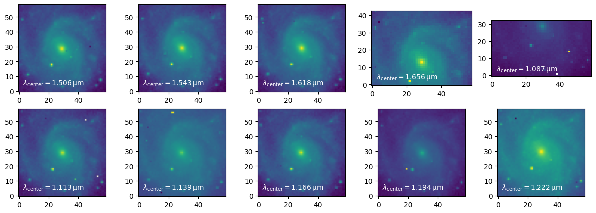
Acknowledgements
About this notebook
Updated: 5 March 2026
Contact: IRSA Helpdesk with questions or problems.
Runtime: As of the date above, this notebook takes about 3 minutes to run to completion on a machine with 8GB RAM and 4 CPU.