Understanding and Extracting the PSF Extension in a SPHEREx Cutout

1. Learning Goals¶

• Determine how pixels in a SPHEREx cutout map to the pixels in the parent SPHEREx spectral image.
• Understand the structure of the PSF extension in a SPHEREx cutout (which is the same as the PSF extension in the parent spectral image)
• Learn which plane in a SPHEREx cutout PSF extension cube most accurately describes the coordinates you are interested in.

2. SPHEREx Overview¶

SPHEREx is a NASA Astrophysics Medium Explorer mission that launched in March 2025. During its planned two-year mission, SPHEREx will obtain 0.75-5 micron spectroscopy over the entire sky, with deeper data in the SPHEREx Deep Fields. SPHEREx data will be used to:

• constrain the physics of inflation by measuring its imprints on the three-dimensional large-scale distribution of matter,
• trace the history of galactic light production through a deep multi-band measurement of large-scale clustering,
• investigate the abundance and composition of water and biogenic ices in the early phases of star and planetary disk formation.

The community will also mine SPHEREx data and combine it with synergistic data sets to address a variety of additional topics in astrophysics.

More information is available in the SPHEREx Explanatory Supplement.

3. Imports¶

The following packages must be installed to run this notebook.

# Uncomment the next line to install dependencies if needed.
# !pip install astropy numpy pyvo

import re
import time

import astropy.units as u
import matplotlib.pyplot as plt
import numpy as np
import pyvo
from astropy.coordinates import SkyCoord
from astropy.io import fits
from astropy.table import Table
from astropy.wcs import WCS

4. Get SPHEREx Cutout¶

We first obtain a SPHEREx cutout for a given coordinate of interest from IRSA archive. For this we define a coordinate and a size of the cutout. Both should be defined using astropy units. The goal is to obtain the cutout and then extract the PSF corresponding to the coordinates of interest.

ra = 305.59875000000005 * u.degree
dec = 41.14888888888889 * u.degree
size = 0.01 * u.degree

Once we defined the coordinates of interest and the size of the cutout, we run a TAP query to gather all SPHEREx spectral images that cover the coordinates.

# Define the service endpoint for IRSA's Table Access Protocol (TAP)
# so that we can query SPHEREx metadata tables.
service = pyvo.dal.TAPService("https://irsa.ipac.caltech.edu/TAP")

# Define a query that will search the appropriate SPHEREx metadata tables
# for spectral images that cover the chosen coordinates of interest.
# Return the cutout data access URL and the time of observation.
# Sort by observation time.
query = f"""
SELECT
    'https://irsa.ipac.caltech.edu/' || a.uri || '?center={ra.to(u.degree).value},{dec.to(u.degree).value}d&size={size.to(u.degree).value}' AS uri,
    p.time_bounds_lower
FROM spherex.artifact a
JOIN spherex.plane p ON a.planeid = p.planeid
WHERE 1 = CONTAINS(POINT('ICRS', {ra.to(u.degree).value}, {dec.to(u.degree).value}), p.poly)
ORDER BY p.time_bounds_lower
"""

# Execute the query and return as an astropy Table.
t1 = time.time()
results = service.search(query)
print("Time to do TAP query: {:2.2f} seconds.".format(time.time() - t1))
print("Number of images found: {}".format(len(results)))

Time to do TAP query: 3.82 seconds.
Number of images found: 173

For this example, we focus on the first one of the retrieved SPHEREx spectral images.

spectral_image_url = results['uri'][0]
print(spectral_image_url)

https://irsa.ipac.caltech.edu/ibe/data/spherex/qr/level2/2025W18_1B/l2b-v13-2025-198/4/level2_2025W18_1B_0023_2D4_spx_l2b-v13-2025-198.fits?center=305.59875000000005,41.14888888888889d&size=0.01

5. Read in a SPHEREx Cutout¶

Next, we use standard astropy tools to open the fits image and to read the different headers and data.

with fits.open(spectral_image_url) as hdul:
    hdul.info()
    cutout_header = hdul['IMAGE'].header
    psf_header = hdul['PSF'].header
    cutout = hdul['IMAGE'].data
    psfcube = hdul['PSF'].data

Filename: /home/runner/.astropy/cache/download/url/87815b4bdf2a8de16d5f6006bbe63e68/contents
No.    Name      Ver    Type      Cards   Dimensions   Format
  0  PRIMARY       1 PrimaryHDU       5   ()      
  1  IMAGE         1 ImageHDU       217   (6, 6)   float32   
  2  FLAGS         1 ImageHDU       146   (6, 6)   int32   
  3  VARIANCE      1 ImageHDU       119   (6, 6)   float32   
  4  ZODI          1 ImageHDU       119   (6, 6)   float32   
  5  PSF           1 ImageHDU       509   (101, 101, 121)   float32   
  6  WCS-WAVE      1 BinTableHDU     18   1R x 3C   [13J, 13J, 338E]   

The downloaded SPHEREx image cutout contains 5 FITS layers, which are described in the SPHEREx Explanatory Supplement. We focus in this example on the extensions IMAGE and PSF. We have already loaded their data as well as their header.

psfcube.shape

The shape of the psfcube is (121,101,101). This corresponds to a grid of 11x11 PSFs across the image, each of them of the size 101x101 pixels.

Let’s look at a small part of the PSF header to understand its format:

psf_header[22:40]

We confirm that the oversampling factor (OVERSAMP) is 10. The PSFs are distributed in an even grid with 11x11 zones. Each of the 121 PSFs is responsible for one of these zones. The PSF header therefore includes the center position of these zones as well as the width of the zones. These center coordinate are specified with XCTR_i and YCTR_i, respectively, where i = 1...121. The widths are specified with XWID_i and YWID_i, respectively, where again i = 1...121. The zones have equal widths and are arranged in an even grid. In principle, the zones can have any size, but this arrangement is enough to capture well the changes of the PSF size and structure with wavelength and spatial coordinates.

The goal of this tutorial now is to find the PSF corresponding to our input coordinates of interest.

6. Determine the Pixel Location on the Parent SPHEREx Image¶

To identify the zone which covers the coordinates of interest, we first need to translate these coordinates to the pixel coordinates on the parent large SPHEREx image from which the cutout was created.

We do this by first determining the pixel (x,y) coordinates of our coordinates of interest on the cutout itself.

wcs = WCS(cutout_header)
xpix_cutout, ypix_cutout = wcs.world_to_pixel(SkyCoord(ra=ra.to(u.degree), dec=dec.to(u.degree)))

print(f"Pixel values of coordinates of interest on cutout image: x = {xpix_cutout}, y = {ypix_cutout}")

Pixel values of coordinates of interest on cutout image: x = 2.1804670006787834, y = 2.341315802366015

Next, we use the CRPIX1A and CRPIX1A header keywords (which describe the center of the cutout on the parent SPHEREx image) to shift the (x,y) coordinates of input to the parent SPHEREx image.

crpix1a = cutout_header["CRPIX1A"]
crpix2a = cutout_header["CRPIX2A"]

xpix_orig = 1 + xpix_cutout - crpix1a
ypix_orig = 1 + ypix_cutout - crpix2a

print(f"Pixel values of coordinates of interest on parent SPHEREx image: x = {xpix_orig}, y = {ypix_orig}")

Pixel values of coordinates of interest on parent SPHEREx image: x = 223.1804670006788, y = 2007.3413158023661

7. Determine the PSF Corresponding to Coordinates of Interest¶

Since we now know the (x,y) pixel values of the coordinates of interest on the parent SPHEREx image, we can identify the PSF zone. In the following we first extract the zone pixel coordinates from the XCTR_* and YCTR_* keys in the PSF header.

xctr = {}
yctr = {}

for key, val in psf_header.items():
    # Look for keys like XCTR* or YCTR*
    xm = re.match(r'(XCTR*)', key)
    if xm:
        xplane = int(key.split("_")[1])
        xctr[xplane] = val
    ym = re.match(r'(YCTR*)', key)
    if ym:
        yplane = int(key.split("_")[1])
        yctr[xplane] = val

Check that we got all of them!

len(xctr) == len(yctr)

Make a nice table so we can easily search for the distance between zone center and coordinates of interest.

tab = Table(names=["zone_id" , "x" , "y"], dtype=[int, float, float])
for zone_id in xctr.keys():
    tab.add_row([zone_id , xctr[zone_id] , yctr[zone_id]])

Once we have created this dictionary with zone pixel coordinates, we can simply search for the closest zone center to the coordinates of interest. For this we first add the distance between zone center coordinates and coordinates of interest to the table

tab["distance"] = np.sqrt((tab["x"] - xpix_orig)**2 + (tab["y"] - ypix_orig)**2)

Then we can sort the table and pick the closest zone to coordinates of interest.

tab.sort("distance")

psf_cube_plane = tab[0]["zone_id"]
distance_min = tab[0]["distance"]

print(f"The PSF zone corresponding to coordinates of interest is {psf_cube_plane} with a distance of {distance_min} pixels")

The PSF zone corresponding to coordinates of interest is 22 with a distance of 81.41754554436464 pixels

8. Extract and Show the PSF¶

Now that we know which zone corresponds to coordinates of interest, we can extract it and plot it.

psf = psfcube[psf_cube_plane]

fig = plt.figure(figsize=(5, 5))
ax1 = fig.add_subplot(1, 1, 1)

ax1.imshow(psf)

plt.show()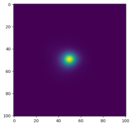

Acknowledgements¶

• Caltech/IPAC-IRSA

About this notebook¶

Authors: IRSA Data Science Team, including Vandana Desai, Andreas Faisst, Brigitta Sipőcz, Troy Raen

Updated: 2025-09-30

Contact: Contact IRSA Helpdesk with questions or problems.

Runtime: Approximately 30 seconds.