Note
Go to the end to download the full example code.
Getting Started
kete has a few foundational concepts which are important to understand. The most important concepts are related to geometry:
Frames - Reference frame, such as Ecliptic, Equatorial, Galactic.
Vectors - Cartesian vectors with an associated coordinate frame.
States - The name, position, velocity, and epoch for a specific object.
Field of View (FOV) - A patch of sky along with the state of the observer.
Cometary Elements - Orbital elements of an object.
Units of position are in AU and velocity is AU / Day.
Basic Geometry
import kete
import numpy as np
import matplotlib.pyplot as plt

# Lets construct an object circular orbit
# Recall that an object in circular orbit has a speed of sqrt(GM / r) where r is the
# radius of the orbit.
r = 1
epoch = kete.Time.j2000()
speed = np.sqrt(kete.constants.SUN_GM / r)
pos = kete.Vector([0, r, 0], frame=kete.Frames.Equatorial)
vel = kete.Vector([-speed, 0, 0], frame=kete.Frames.Equatorial)

# We now make a State, representing the full information for an object in orbit of the
# sun.
state = kete.State("Circular", epoch, pos, vel)
state
State(desig="Circular", jd=2451545.0, pos=[0.0, 1.0, 0.0], vel=[-0.017202098949957226, 0.0, 0.0], frame=Equatorial, center_id=10)
Vectors have convenient conversions to and from common reference frames:
pos.as_equatorial, pos.as_ecliptic
(Vector([0.0, 1.0, 0.0], Equatorial), Vector([0.0, 0.917482062069, -0.397777155932], Ecliptic))
Creation of vectors also have a few convenient helper functions:
# On sky position of the andromeda galaxy
ra = kete.conversion.ra_hms_to_degrees("0 42 44")
dec = kete.conversion.dec_dms_to_degrees("+41 16 9")
vec = kete.Vector.from_ra_dec(ra, dec)

# Change to galactic frame, and print the elevation and azimuth
vec = vec.change_frame(kete.Frames.Galactic)
vec.el, vec.az
(-21.57285600487441, 121.17322536853838)
Now that we have seen how to make a state, lets look at much easier ways to get this data so that it is not necessary to hand write the position and velocities.
Getting states
There are multiple ways to retrieve state information:
Manual entry, either from orbit elements of direct values.
From Spice (local)
From JPL Horizons (internet)
From the Minor Planet Center (internet)
We have just seen an example of the first way, lets explore the other ways.
# Grabbing the state of the Moon.
# kete includes spice kernels for all of the planets, the Moon, Pluto and 5 asteroids:
# Ceres, Pallas, Vesta, Hygiea, Interamnia
jd = kete.Time.from_ymd(2020, 1, 1).jd
moon = kete.spice.get_state("Moon", jd)

# Grabbing a state from JPL Horizons
# Note that the epoch of this state is the epoch of fit from Horizons.
eros = kete.HorizonsProperties.fetch("Eros").state

# Grabbing a state from the MPC
# This is more expensive, as the MPC lookup involves downloading a full copy of the MPC
# database. This database contains more than a million asteroids. This gets returned as
# a pandas dataframe.
orb_file = kete.mpc.fetch_known_orbit_data()
subset = orb_file[orb_file["name"] == "Eros"]

# Note that in this case the tool converts all objects in the provided table into states
# which means it will always return a list of states, so below we get a list containing
# a single state.
states = kete.mpc.table_to_states(subset)
states
[State(desig="433", jd=2461000.500800741, pos=[0.8031182010894415, 0.9930974783800428, 0.23391023935572156], vel=[-0.013933047915076657, 0.007535954903271381, -0.001390705835268776], frame=Ecliptic, center_id=10)]
Moving states
The state(s) which are constructed above usually do not have an epoch which is useful. Luckily, kete has tools for propagating the states forward and backward in time to whichever epoch is desired. There are 2 workhorse functions related to orbit propagation:
- propagate_n_body
Highest accuracy, propagate a list of States to the desired Time using full orbital mechanics including all planets, and optionally the 5 largest asteroids. This includes effects due to General Relativity, and the non-spherical J2 term of Jupiter, the Sun, and Earth. Optionally supports non-gravitational forces such as Solar Radiation Pressure (SRP) and Poynting-Robertson.
- propagate_two_body
Lower accuracy but faster, propagate the orbit using Keplerian mechanics, only including the force due to the Sun.
Both of these functions work on many states at once, and are designed to propagate the entire MPC catalog simultaneously.
# Lets grab the state of a few asteroids:
names = ["Eros", "Bennu", "Ryugu"]

orb_file = kete.mpc.fetch_known_orbit_data()
subset = orb_file[[name in names for name in orb_file["name"]]]

# This now contains 3 states:
states = kete.mpc.table_to_states(subset)

# Lets propagate these states to the current epoch
now = kete.Time.now().jd

states_now_exact = kete.propagate_n_body(states, now)
states_now_kepler = kete.propagate_two_body(states, now)
states_now_exact
[State(desig="433", jd=2461190.6083439933, pos=[-1.1999971525828133, -0.5450296222066658, -0.24838803949019614], vel=[0.003441102063490981, -0.015011914069212966, -0.0010728496409111391], frame=Ecliptic, center_id=10), State(desig="101955", jd=2461190.6083439933, pos=[-0.9737467379071475, 0.43803116335070236, 0.04979790758368652], vel=[-0.009964277094271124, -0.013768520047365305, -0.0014181367884918304], frame=Ecliptic, center_id=10), State(desig="162173", jd=2461190.6083439933, pos=[-1.0879721056625828, 0.03581964196925313, -0.10705989858420735], vel=[-0.003552760642765794, -0.01673106263522077, 0.00020569853535364144], frame=Ecliptic, center_id=10)]
Field of Views
Knowing the state of an object in the solar system is interesting by itself, but unfortunately not directly useful when actually observing. To start with, we have to define the location of the observer. For ground observers, there are 2 simple ways to retrieve this position:
Using an MPC Observatory code
Using Earth based latitude/longitude and altitude as one would find on a map.
now = kete.Time.now().jd

# lookup the observers position in the solar system from a given observatory code/name.
observer_a = kete.spice.mpc_code_to_ecliptic("Palomar Mountain", now)

# lookup the observer position from an earth location, this is IPAC, at 100m altitude.
observer_b = kete.spice.earth_pos_to_ecliptic(now, 33.133278, 241.87206, 0.1, "IPAC")
observer_b
State(desig="IPAC", jd=2461190.608344028, pos=[-0.37383194185010477, -0.942123849906639, 7.983435066906094e-5], vel=[0.015659763610965854, -0.0066071457459665915, 8.808726761812482e-5], frame=Ecliptic, center_id=10)
Now that we have the observer location, we can define a Field of View for that observer. There are many different possible FOVs, the conceptually simplest one is an omni-directional field of view:
fov = kete.OmniDirectionalFOV(observer_a)
fov
OmniDirectional(observer=State(desig="675", jd=2461190.608344028, pos=[-0.37383201929853394, -0.9421245166356763, 8.027930104898072e-5], vel=[0.015664732756290493, -0.006607600656303284, 8.827054776004417e-5], frame=Ecliptic, center_id=10))
We can now compute the observed position of objects in this FOV:
state = kete.HorizonsProperties.fetch("Eros").state

# This accepts many states and many FOVs at once, it is the most efficient when all the
# requested states and FOVs are provided at the same time.
visible = kete.fov_state_check([state], [fov])[0]
visible
SimultaneousStates(states=<1 States>, fov=OmniDirectional(observer=State(desig="675", jd=2461190.608344028, pos=[-0.37383201929853394, -0.9421245166356763, 8.027930104898072e-5], vel=[0.015664732756290493, -0.006607600656303284, 8.827054776004417e-5], frame=Ecliptic, center_id=10)))
The returned object requires some discussion, as it has not been covered yet. fov_state_check returns a SimultaneousState, which is a collection of States which are at the same epoch, along with an optional FOV. If the FOV is present, it is assumed that the states are the location as seen from the observers location along with the effects of light delay.
If the FOV is provided, as it would be after the fov_state_check call will do, then there is a function on the SimultaneousState which provides the vectors from the observer to the objects.
obs_vecs = visible.obs_vecs[0]
obs_vecs = obs_vecs.as_equatorial
obs_vecs.ra, obs_vecs.dec
(150.72144745514535, -4.2253136261887505)
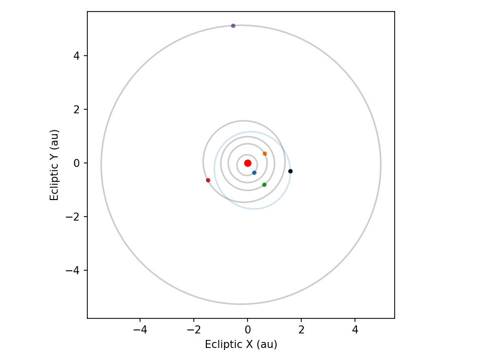
Plotting Planets
Here is a basic example of using kete to plot an orbit.
plt.figure(dpi=150)
jd = kete.Time.now().jd
plt.gca().set_aspect("equal", "box")

# plot the planets orbits
for i, planet in enumerate(["Mercury", "Venus", "Earth", "Mars", "Jupiter"]):
    plan = kete.spice.get_state(planet, jd)
    plt.scatter(plan.pos.x, plan.pos.y, color=f"C{i}", s=10)
    jds = np.linspace(jd - plan.elements.orbital_period, jd, 100)
    pos = np.array([kete.spice.get_state(planet, jd).pos for jd in jds]).T
    plt.plot(pos[0], pos[1], color="black", alpha=0.2)

# plot the orbit of eros, using 2 body mechanics to plot the previous orbit
eros = kete.HorizonsProperties.fetch("Eros").state
eros = kete.propagate_two_body([eros], jd)[0]
plt.scatter(eros.pos.x, eros.pos.y, c="black", s=10)
jds = np.linspace(jd - eros.elements.orbital_period, jd, 100)
pos = np.array([kete.propagate_two_body([eros], jd)[0].pos for jd in jds]).T
plt.plot(pos[0], pos[1], c="C0", alpha=0.2)

plt.xlabel("Ecliptic X (au)")
plt.ylabel("Ecliptic Y (au)")
plt.scatter(0, 0, color="red")
plt.tight_layout()
plt.show()
Total running time of the script: (0 minutes 0.656 seconds)