1. Learning Goals
Open a SPHEREx HiPS All-Sky Mosaic in Firefly starting from a Jupyter Notebook.
Select a specific HiPS Mosaic layer related to a specific wavelength.
Download the FITS cube corresponding to a specific HealPix for a given position on sky.
Extract a quick look spectrum from the FITS cube at a given position.
2. SPHEREx Overview
SPHEREx is a NASA Astrophysics Medium Explorer mission that launched in March 2025. During its planned two-year mission, SPHEREx will obtain 0.75-5 micron spectroscopy over the entire sky, with deeper data in the SPHEREx Deep Fields. SPHEREx data will be used to:
constrain the physics of inflation by measuring its imprints on the three-dimensional large-scale distribution of matter,
trace the history of galactic light production through a deep multi-band measurement of large-scale clustering,
investigate the abundance and composition of water and biogenic ices in the early phases of star and planetary disk formation.
The community will also mine SPHEREx data and combine it with synergistic data sets to address a variety of additional topics in astrophysics.
More information is available in the SPHEREx Explanatory Supplement.
3. Imports
The following packages must be installed to run this notebook.
# Uncomment the next line to install dependencies if needed.
# !pip install astropy matplotlib numpy photutils hpgeom requests firefly_client
import os
import io
import warnings
import numpy as np
import posixpath
from astropy.io import fits
from astropy.table import Table, vstack
from astropy.stats import SigmaClip
from astropy.wcs import WCS
from astropy.coordinates import SkyCoord
import astropy.units as u
from astropy.io.votable import from_table
from astropy.io.votable.tree import Group, FieldRef
from photutils.aperture import CircularAperture, CircularAnnulus, ApertureStats, aperture_photometry
import hpgeom as hp
import requests
from firefly_client import FireflyClient
import matplotlib.pyplot as plt
import matplotlib as mpl
import matplotlib.transforms as mtransforms/home/runner/work/irsa-tutorials/irsa-tutorials/.tox/py312-buildhtml/lib/python3.12/site-packages/tqdm/auto.py:21: TqdmWarning: IProgress not found. Please update jupyter and ipywidgets. See https://ipywidgets.readthedocs.io/en/stable/user_install.html
from .autonotebook import tqdm as notebook_tqdm
## Define some plotting formats
def load_plotting_defaults():
    mpl.rcParams['xtick.minor.visible'] = True
    mpl.rcParams['ytick.minor.visible'] = True
    mpl.rcParams['xtick.minor.top'] = True
    mpl.rcParams['xtick.minor.bottom'] = True
    mpl.rcParams['ytick.minor.left'] = True
    mpl.rcParams['ytick.minor.right'] = True
    mpl.rcParams['xtick.major.size'] = 5
    mpl.rcParams['ytick.major.size'] = 5
    mpl.rcParams['xtick.minor.size'] = 3
    mpl.rcParams['ytick.minor.size'] = 3
    mpl.rcParams['xtick.direction'] = 'in'
    mpl.rcParams['ytick.direction'] = 'in'
    mpl.rcParams['xtick.top'] = True
    mpl.rcParams['ytick.right'] = True
    mpl.rc('font', family='sans-serif')

load_plotting_defaults()
def_cols = plt.rcParams['axes.prop_cycle'].by_key()['color']
4. Understanding the HiPS All-Sky Mosaic Cube
We first spend some time to understand the format of the HiPS All-Sky Mosaic Cube. To interact with the cube, we need an URL where it is hosted. There are two URLs:
The first one (hereafter
hips_url) links to the AllSky Cube that FireFly will use. We feed this URL to Firefly (Section 5)The second one (hereafter
hips_data_url) links to the data behind the AllSky Cube. This URL is used when we access the FITS cube directly (Section 6)
hips_url = "https://irsa.ipac.caltech.edu/data/hips/SPHEREx/spherex_allsky_cube"
hips_data_url = "https://irsa.ipac.caltech.edu/ibe/data/spherex/dr1/hips5_cube/hips_20261026"
We can first load the HiPS properties from the properties metadata. For this, we have to retrieve the HiPS from the above URL. We do this by using the requests library.
response = requests.get(f"{hips_url}/properties")
response.raise_for_status()
Once loaded, we can create a property dictionary.
properties = {}
for line in response.text.splitlines():
    line = line.strip()
    if not line or line.startswith("#"):
        continue
    if "=" in line:
        key, value = line.split("=", 1)
        properties[key.strip()] = value.strip()
From the properties, we can print the description of the HiPS mosaic cube for more information.
properties["obs_description"]'SPHEREx DR1 all-sky data cube for visualization: 102 frames in ascending wavelength, one per band (1-6) and channel (1-17), frame index = 17*(band-1) + (channel-1). Frames 50 and 51 (band 3 channel 17, band 4 channel 1, the dichroic channels) are blank. See the SPHEREx Explanatory Supplement: https://irsa.ipac.caltech.edu/data/SPHEREx/docs/SPHEREx_Expsupp.pdf'Another important property is the wavelength encoding of the cube layers. Let’s load these in a nice table.
wavetab = Table([
                np.asarray(properties["data_cube_crval3_arr"].split(" ")).astype(float)*u.micrometer,
                np.arange(int(properties["hips_cube_depth"]))
             ],
                names=["lambda_um","layer_id"])

wavetab[0:10]We see that each HiPS cube has 102 wavelength layers, which we have linked to wavelengths (in ) in the table wavetab. Next, we use Firefly to visualize the All-Sky HiPS mosaic cube.
5. HiPS All-Sky Cube in Firefly
We first demonstrate how we can use Firefly to open and explore an All-Sky HiPS mosaic cube. For this, we first have to define the URL of the HiPS cube. This will then be loaded in Firefly.
First, let’s define some coordinates. These are later used to center the Firefly visualization and also retrieve the FITS cube.
ra = 60.8109955*u.degree
dec = 51.3404038*u.degree
Now start the Firefly server.
fc = FireflyClient.make_client(url="https://irsa.ipac.caltech.edu/irsaviewer")Now, we open the HiPS All-Sky Mosaic Cube in Firefly. We can also define the field of view of the visualizer.
hips_plot_id = 'spherex_cube' # to identify this particular image display for later operations

fov_degree = 10*u.degree

fc.show_hips(plot_id=hips_plot_id,
             hips_root_url=hips_url,
             Title='HiPS image',
             WorldPt=f'{ra.to_value(u.degree)};{dec.to_value(u.degree)};EQ_J2000',
             SizeInDeg=fov_degree.to_value(u.degree) # can be omitted
             )
{'success': True}Let’s choose a wavelength to center the cube layer on.
lambda_view = 3.3*u.micrometer... and select the correct layer.
idx = np.argmin(np.abs(wavetab["lambda_um"] - lambda_view.to_value(u.micrometer)))
layer_view = int(wavetab["layer_id"][idx])
print(f"Wavelength {lambda_view} is closest to layer {layer_view}")
Wavelength 3.3 um is closest to layer 62
With this separate dispatch, we can choose the wavelength layer.
Now that we know the layer that connects to the chosen wavelength, we can send an additional dispatch to Firefly to open the layer corresponding to the chosen wavelength.
fc.dispatch(action_type='ImagePlotCntlr.ChangeHiPS',
            payload={'plotId': f"{hips_plot_id}", 'cubeIdx': layer_view}) # plotId needs to be same as what you passed in show_hips() and cubeIdx is 0-based
{'success': True}6. Download and Display HiPS FITS Cube
6.1 Download HiPS FITS Cube
Next, we show how to download a HiPS cube in FITS format for a given Healpix pixel. For this, we first have to find the Healpix pixel corresponding to our coordinates. Then we have to construct the URL to the corresponding FITS cube, which we then can load using the astropy package.
To find the Healpix pixel corresponding to the R.A./Decl. coordinates, we make use of the healpy package (which we imported above). Note that we are assuming her HiPS order 5, which is the smallest scale that is supported by the current SPHEREx All-Sky Mosaic. But in principle, you can choose an order, if available. We can directly check the properties dictionary that we have created above to find out what the minimum and maximum HiPS order is:
print(f"Minimum HiPS order (largest spatial scale): {properties['hips_order_min']}")
print(f"Maximum HiPS order (smallest spatial scale): {properties['hips_order']}")
Minimum HiPS order (largest spatial scale): 0
Maximum HiPS order (smallest spatial scale): 5
Choose Norder:
Norder = 5Finally get the Healpix pixel number corresponding to our search coordinates.
nside = 2**Norder
ipix = hp.angle_to_pixel(nside, ra.to_value(u.degree), dec.to_value(u.degree), nest=True, lonlat=True)
print(f"Healpix pixel number corresponding to R.A. = {ra} and Decl. = {dec}: {ipix}")
Healpix pixel number corresponding to R.A. = 60.8109955 deg and Decl. = 51.3404038 deg: 445
Now that we know the Healpix pixel number, we can construct the URL leading to the FITS cube.
dirid = (ipix // 10000) * 10000
#cube_url = posixpath.join(hips_data_url, f"Norder{Norder}", f"Dir{dirid}", f"Npix{ipix}", f"Npix{ipix}_cube.fits")
cube_url = posixpath.join(hips_data_url, f"Norder{Norder}", f"Dir{dirid}", f"Npix{ipix}_cube.fits")
print(f"Cube URL: {cube_url}")
Cube URL: https://irsa.ipac.caltech.edu/ibe/data/spherex/dr1/hips5_cube/hips_20261026/Norder5/Dir0/Npix445_cube.fits
Once we have the cube URL, we can load the FITS cube directly.
6.2 Display HiPS FITS Cube
Next, we demonstrate how to load the FITS cube and how to display a specific layer of it.
The SPHEREx HiPS FITS cube consists of different extensions.
The
IMAGEextension is the actual science cubeThe
NHITSextension shows the number of contributing input pixels per mosaic pixel.The
FLAGSextension includes bitwise OR of flags propagated from contributing input pixels.
For more information on these layer and the FITS cube construction, we refer to the “Mosaics” Section of the SPHEREx Explanatory Supplement.
First, we open the FITS cube using the cube_url that we have defined above.
with fits.open(cube_url, cache=False) as hdul:
    hdul.info()
    img_cube = hdul["IMAGE"].data ## image cube
    img_hdr = hdul["IMAGE"].header ## image cube header
    hits_cube = hdul["NHITS"].data ## hits cube
    hits_hdr = hdul["NHITS"].header ## hits cube header
    flags_cube = hdul["FLAGS"].data ## flags cube
    flags_hdr = hdul["FLAGS"].header ## flags cube
    wcs_img = WCS(hdul["IMAGE"].header, fobj=hdul) ## WCS
    spec_channels = Table.read(hdul["SPECTRAL_CHANNELS"], cache=False) ## spectral channel table
Filename: /tmp/astropy-download-4942-1tezud1k
No. Name Ver Type Cards Dimensions Format
0 PRIMARY 1 PrimaryHDU 15 ()
1 IMAGE 1 ImageHDU 47 (512, 512, 102) float32
2 NHITS 1 ImageHDU 47 (512, 512, 102) int32
3 FLAGS 1 ImageHDU 114 (512, 512, 102) int32
4 SPECTRAL_CHANNELS 1 BinTableHDU 35 102R x 8C [I, I, E, E, E, E, E, E]
5 WCS-WAVE 1 BinTableHDU 18 1R x 3C [102J, 102E, 102E]
Let’s first check the dimensions of the cube. It should have 102 layers, corresponding to the wavelengths.
print(f"Cube shape: {img_cube.shape}")Cube shape: (102, 512, 512)
In addition, we can also read in the spectral channels table, that contains more information on the wavelength of the channels and their widths. Let’s look at it here.
spec_channels[0:10]Let’s select again the same layers corresponding to the wavelength we want and plot the image. We extract the 2D image, hit map, and flag map at the requested layer.
img = img_cube[layer_view, :, :]
hits = hits_cube[layer_view, :, :]
flags = flags_cube[layer_view, :, :]
Finally plot the image with the coordinates indicated. Note that we have to use the WCS transformation here.
fig = plt.figure(figsize=(18,6))
ax1 = fig.add_subplot(1,3,1, projection=wcs_img.celestial) # image
ax2 = fig.add_subplot(1,3,2, projection=wcs_img.celestial) # hit map
ax3 = fig.add_subplot(1,3,3, projection=wcs_img.celestial) # flags map

## Plot the image
im1 = ax1.imshow(img, origin="lower", norm="log", cmap="viridis")
ax1.plot(ra, dec, "o", markersize=10, fillstyle="none", markeredgecolor="red", transform=ax1.get_transform("world"))
ax1.set_title("Science Image")

## Plot the hit map
im2 = ax2.imshow(hits, origin="lower", norm="linear", cmap="Greys")
ax2.plot(ra, dec, "o", markersize=10, fillstyle="none", markeredgecolor="red", transform=ax2.get_transform("world"))
ax2.set_title("Hits Map")

## Plot the flags map
im3 = ax3.imshow(flags, origin="lower", norm="linear", cmap="Greys")
ax3.plot(ra, dec, "o", markersize=10, fillstyle="none", markeredgecolor="red", transform=ax3.get_transform("world"))
ax3.set_title("Flags Map")


## Axes
for ax,im in zip([ax1,ax2,ax3], [im1,im2,im3]):
    ax.set_xlabel("RA")
    ax.set_ylabel("Dec")
    ax.coords.grid(color="white", alpha=0.8, ls="dotted")
    plt.colorbar(im, ax=ax, orientation="vertical", location="right", shrink=0.8)

plt.show()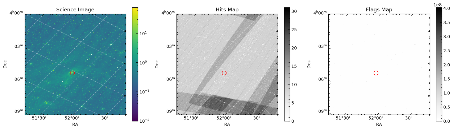
6.3 Drill Through the FITS Cube
We can extract a very basic spectrum directly from the FITS cube.
To obtain the spectrum, we create a function that computes the sum of the fluxes in apertures and does a background subtraction using an annulus. Both aperture and annulus sizes are user-defined. We use the PhotUtils package for this (see here for more information).
The measurements are done for each cube plane and the combined.
Furthermore, the function creates a plot showing the collapsed cube and the apertures used (this output can be turned off).
def local_pixel_scale(wcs_cel, x, y):
    '''
    Effective angular size of one pixel at pixel position (x, y), as the square
    root of the local pixel solid angle. This is measured on the sky, so it is
    correct for projections like HPX whose projection plane is not to scale.

    Returns
    -------
    astropy.units.Quantity
        Pixel scale in arcsec / pixel.
    '''
    c0, c1, c2 = wcs_cel.pixel_to_world([x, x + 1, x], [y, y, y + 1])
    dlon1, dlat1 = c0.spherical_offsets_to(c1)
    dlon2, dlat2 = c0.spherical_offsets_to(c2)
    area = np.abs(dlon1 * dlat2 - dlat1 * dlon2)
    return np.sqrt(area).to(u.arcsec) / u.pixel


def aperture_sum_to_mjy(aperture_sum, pixscale, bunit=u.MJy / u.sr):
    '''
    Convert an aperture sum of a surface-brightness image (summed over pixels)
    into a flux density in mJy.

    Parameters
    ----------
    aperture_sum : array-like
        Sum of pixel values inside the aperture, in units of `bunit` per pixel.
    pixscale : astropy.units.Quantity
        Pixel scale (angle / pixel), e.g. from `local_pixel_scale`.
    bunit : astropy.units.Unit
        Surface-brightness unit of the image (default MJy/sr).

    Returns
    -------
    astropy.units.Quantity
        Flux density in mJy.
    '''
    pix_sr = ((pixscale * u.pixel) ** 2).to(u.sr)
    return (np.asarray(aperture_sum) * u.Unit(bunit) * pix_sr).to(u.mJy)


def _radius_to_pixels(r, name, pixscale):
    '''
    Convert a radius given in pixels or an angular unit to a float number of pixels.
    Plain numbers are interpreted as pixels.
    '''
    if not isinstance(r, u.Quantity):
        return float(r)
    if r.unit.is_equivalent(u.pixel):
        return float(r.to_value(u.pixel))
    if r.unit.is_equivalent(u.arcsec):
        if pixscale is None:
            raise ValueError(f"`{name}` is given in angular units ({r.unit}), "
                             "which requires a `wcs` to convert to pixels.")
        return float((r / pixscale).to_value(u.pixel))
    raise u.UnitsError(f"`{name}` must be in pixels or angular units, got {r.unit}.")


def measure_aperture_photometry_cube(cube, *, ra=None, dec=None, wcs=None,
                                     r_aperture=20 * u.pixel,
                                     r_inner=60 * u.pixel,
                                     r_outer=100 * u.pixel,
                                     bunit=u.MJy / u.sr,
                                     makeplot=True):
    '''
    Create quick look spectrum from simple aperture photometry with background
    subtraction from annulus.

    Parameters
    ----------
    cube : numpy.ndarray
        Input SPHEREx mosaic cube with shape (n_planes, ny, nx).
    ra, dec : float or astropy.units.Quantity, optional
        Sky position at which to extract the photometry. Floats are interpreted
        as degrees. If not given, the center of the cube is used.
    wcs : astropy.wcs.WCS, optional
        WCS of the cube. Required if `ra` and `dec` are given, or if any radius
        is given in angular units. Can be the 2D celestial WCS or a
        higher-dimensional WCS (its celestial part is used). If given, it is
        also used to draw RA/Dec axes in the plot.
    r_aperture : astropy.units.Quantity or float
        Aperture radius for flux extraction, in pixels (u.pixel) or any angular
        unit (e.g. u.arcsec). Plain numbers are interpreted as pixels.
    r_inner : astropy.units.Quantity or float
        Inner radius of the background annulus (pixels or angular units).
    r_outer : astropy.units.Quantity or float
        Outer radius of the background annulus (pixels or angular units).
    bunit : astropy.units.Unit
        Surface-brightness unit of the cube (default MJy/sr). Used to convert
        the aperture sums to flux densities in mJy (requires `wcs`).
    makeplot : bool
        Set to `True` if function should create a figure showing the collapsed
        cube with overlay of aperture and annuli.

    Returns
    -------
    astropy.table.QTable
        A table including the photometry results (sum of aperture flux, plane ID,
        etc). `aperture_sum` and `aperture_sum_bkgsub` are sums of pixel values
        (`bunit` x pixels). If a `wcs` is given, `flux_mjy` and `flux_bkgsub_mjy`
        hold the corresponding flux densities in mJy. The radii used (in pixels and arcsec) and the pixel scale are
        stored in the table's `meta`.
    '''

    ## Define helper function to compute the photometry efficiently
    def apphot_helper(img, aperture, annulus_aperture):
        '''
        Compute background-subtracted aperture photometry for a single 2D image.
        '''
        ## Calculate background
        sigclip = SigmaClip(sigma=3.0, maxiters=10)
        aperstats = ApertureStats(img, annulus_aperture, sigma_clip=sigclip)
        bkg_mean = aperstats.mean
        aperture_area = aperture.area_overlap(img)
        total_bkg = bkg_mean * aperture_area

        ## Get photometry and subtract background
        phot_table = aperture_photometry(img, aperture)
        phot_table["aperture_sum_bkgsub"] = phot_table["aperture_sum"] - total_bkg

        return phot_table

    ny, nx = cube.shape[1], cube.shape[2]

    ## Celestial part of the WCS (works for 2D or N-D input)
    wcs_cel = None
    if wcs is not None:
        wcs_cel = wcs.celestial if wcs.naxis > 2 else wcs

    ## Define position (photutils expects (x, y) = (column, row), 0-based)
    if (ra is None) != (dec is None):
        raise ValueError("Give both `ra` and `dec`, or neither.")

    if ra is not None:
        if wcs_cel is None:
            raise ValueError("A `wcs` is required when `ra` and `dec` are given.")
        coord = SkyCoord(u.Quantity(ra, u.deg), u.Quantity(dec, u.deg), frame="icrs")
        x, y = wcs_cel.world_to_pixel(coord)
        x, y = float(x), float(y)

        if not (np.isfinite(x) and np.isfinite(y)):
            raise ValueError(f"RA/Dec ({coord.ra.deg:.5f}, {coord.dec.deg:.5f}) "
                             "could not be converted to a pixel position.")
        if not (-0.5 <= x <= nx - 0.5 and -0.5 <= y <= ny - 0.5):
            raise ValueError(f"RA/Dec ({coord.ra.deg:.5f}, {coord.dec.deg:.5f}) falls at "
                             f"pixel ({x:.1f}, {y:.1f}), outside the cube ({nx} x {ny}).")
    else:
        x, y = (nx - 1) / 2, (ny - 1) / 2

    position = (x, y)

    ## Convert radii to pixels, using the pixel scale at the extraction position
    pixscale = local_pixel_scale(wcs_cel, x, y) if wcs_cel is not None else None
    r_ap_px = _radius_to_pixels(r_aperture, "r_aperture", pixscale)
    r_in_px = _radius_to_pixels(r_inner, "r_inner", pixscale)
    r_out_px = _radius_to_pixels(r_outer, "r_outer", pixscale)

    if not (0 < r_ap_px and 0 < r_in_px < r_out_px):
        raise ValueError("Radii must be positive and r_inner < r_outer "
                         f"(got {r_ap_px:.2f}, {r_in_px:.2f}, {r_out_px:.2f} px).")
    if r_ap_px > r_in_px:
        warnings.warn("The aperture is larger than the inner annulus radius, "
                      "so the background annulus overlaps the source aperture.")

    ## Warn if the apertures run off the edge of the image
    if (x - r_out_px < -0.5 or x + r_out_px > nx - 0.5
            or y - r_out_px < -0.5 or y + r_out_px > ny - 0.5):
        warnings.warn("The background annulus extends beyond the image edge; "
                      "background is estimated from the part inside the image only.")

    aperture = CircularAperture(position, r=r_ap_px)
    annulus_aperture = CircularAnnulus(position, r_in=r_in_px, r_out=r_out_px)

    ## Compute photometry (use helper function to iterate over planes)
    phot_all = vstack([apphot_helper(cube[ii, :, :], aperture, annulus_aperture)
                       for ii in range(cube.shape[0])])
    phot_all["id"] = np.arange(cube.shape[0]) + 0  ## add plane numbers back (0-based)
    phot_all.rename_column("id", "plane")

    ## Convert aperture sums (bunit x pixels) to flux densities in mJy
    sum_unit = u.Unit(bunit) * u.pixel
    if pixscale is not None:
        phot_all["flux_mjy"] = aperture_sum_to_mjy(phot_all["aperture_sum"], pixscale, bunit)
        phot_all["flux_bkgsub_mjy"] = aperture_sum_to_mjy(phot_all["aperture_sum_bkgsub"],
                                                          pixscale, bunit)
    else:
        warnings.warn("No `wcs` given, so the pixel solid angle is unknown and "
                      "fluxes in mJy are not computed.")
    phot_all["aperture_sum"].unit = sum_unit
    phot_all["aperture_sum_bkgsub"].unit = sum_unit

    ## Record what was actually used
    if ra is not None:
        phot_all.meta["ra_deg"] = coord.ra.deg
        phot_all.meta["dec_deg"] = coord.dec.deg
    phot_all.meta["r_aperture_px"] = r_ap_px
    phot_all.meta["r_inner_px"] = r_in_px
    phot_all.meta["r_outer_px"] = r_out_px
    if pixscale is not None:
        phot_all.meta["pixscale_arcsec"] = pixscale.to_value(u.arcsec / u.pixel)
        phot_all.meta["r_aperture_arcsec"] = r_ap_px * phot_all.meta["pixscale_arcsec"]
        phot_all.meta["r_inner_arcsec"] = r_in_px * phot_all.meta["pixscale_arcsec"]
        phot_all.meta["r_outer_arcsec"] = r_out_px * phot_all.meta["pixscale_arcsec"]

    ## Plot if asked for
    if makeplot:
        fig = plt.figure(figsize=(5, 5))
        if wcs_cel is not None:
            ax1 = fig.add_subplot(1, 1, 1, projection=wcs_cel)
        else:
            ax1 = fig.add_subplot(1, 1, 1)

        # Plot the median image
        img_plot = np.nanmedian(cube, axis=0)
        possel = img_plot[np.isfinite(img_plot) & (img_plot > 0)]
        lims = np.nanpercentile(possel.flatten(), q=(5, 99.9))
        ax1.imshow(img_plot, origin="lower", vmin=lims[0], vmax=lims[1],
                   norm="log", cmap="inferno")

        # Plot the extraction position
        ax1.plot(x, y, "+", color="white")

        # Plot the apertures
        aperture.plot(ax=ax1, linestyle="-", color="white", label="Aperture")
        annulus_aperture.plot(ax=ax1, linestyle=":", color="white", label="Background")

        ax1.legend(loc="lower right", fontsize=9, framealpha=1,
                   facecolor="black", labelcolor="white")

        if wcs_cel is not None:
            ax1.set_xlabel("RA")
            ax1.set_ylabel("Dec")
        else:
            ax1.tick_params(which="both", axis="both", color="white", labelsize=11)
            ax1.set_xlabel(r"$x$ [px]")
            ax1.set_ylabel(r"$y$ [px]")

        # Keep the view on the cube even if the apertures extend past the edge
        ax1.set_xlim(-0.5, nx - 0.5)
        ax1.set_ylim(-0.5, ny - 0.5)

        plt.show()

    return phot_all
phot_table = measure_aperture_photometry_cube(img_cube, ra=ra, dec=dec, wcs=wcs_img.celestial,
r_aperture=5*u.pixel,
r_inner = 40*u.pixel,
r_outer = 60*u.pixel,
makeplot = True,
bunit = u.Unit(img_hdr["BUNIT"])
)
phot_table["lambda_um"] = spec_channels['WAVELENGTH'].copy()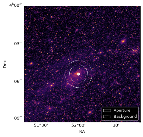
phot_table[0:10]Now that we have extracted the spectrum, let’s plot it. In this tutorial, we have targeted a cloud in the Milky Way, which is characterized by strong Polycyclic Aromatic Hydrocarbon (PAH) emission. We see that in the spectrum that we extracted.
We first define the default lines to plot...
DEFAULT_LINES = [
    (1.282, r"Pa$\beta$"),
    (1.60, r"H$^-$ 1.6$\mu$m"),
    (1.875, r"Pa$\alpha$"),
    (2.166, r"Br$\gamma$"),
    (2.626, r"Br$\beta$"),
    (3.30, r"PAH 3.3"),
    (4.052, r"Br$\alpha$"),
    (4.67, "CO")
]
And then define a handy function to plot the spectrum given the DEFAULT_LINES and the photometry table.
def plot_spectrum(wave, flux, *, bandwidth=None, flux_err=None, lines=DEFAULT_LINES,
                  ax=None, title=None, ylabel="Flux density [mJy]", color="black"):
    '''
    Plot a SPHEREx quick-look spectrum with labelled spectral features.

    Parameters
    ----------
    wave : array-like or Quantity
        Channel center wavelengths (micron if no unit).
    flux : array-like or Quantity
        Flux per channel.
    bandwidth : array-like or Quantity, optional
        Channel widths; drawn as horizontal bars (+/- bandwidth/2).
    flux_err : array-like or Quantity, optional
        Flux uncertainties; drawn as vertical error bars.
    lines : list of (wavelength_um, label)
        Features to mark. Only those inside the plotted range are drawn.
        Pass [] to draw none.
    ax : matplotlib Axes, optional
        Axes to draw into; a new figure is created if omitted.

    Returns
    -------
    fig, ax
    '''
    wave = u.Quantity(wave, u.um).to_value(u.um)
    flux = np.asarray(getattr(flux, "value", flux), dtype=float)
    xerr = None if bandwidth is None else u.Quantity(bandwidth, u.um).to_value(u.um) / 2
    yerr = None if flux_err is None else np.asarray(getattr(flux_err, "value", flux_err))

    order = np.argsort(wave)
    wave, flux = wave[order], flux[order]
    xerr = None if xerr is None else xerr[order]
    yerr = None if yerr is None else yerr[order]

    if ax is None:
        fig, ax = plt.subplots(figsize=(8, 4), layout="constrained")
    else:
        fig = ax.figure

    # Spectrum: thin connecting line, then points with channel widths
    ax.plot(wave, flux, "-", lw=0.8, color=color, alpha=0.35, zorder=2)
    ax.errorbar(wave, flux, xerr=xerr, yerr=yerr, fmt="o", ms=3.5,
                color=color, mfc=color, mec="white", mew=0.4,
                elinewidth=0.6, ecolor=color, alpha=0.9, zorder=3)

    # Axis range with a little padding, and headroom at the top for labels
    pad = 0.02 * (wave.max() - wave.min())
    ax.set_xlim(wave.min() - pad, wave.max() + pad)
    finite = np.isfinite(flux)
    lo, hi = np.nanmin(flux[finite]), np.nanmax(flux[finite])
    span = hi - lo if hi > lo else abs(hi) or 1.0
    ax.set_ylim(lo - 0.08 * span, hi + 0.40 * span)

    # Feature markers: line in data x, label pinned near the top of the axes
    trans = mtransforms.blended_transform_factory(ax.transData, ax.transAxes)
    xmin, xmax = ax.get_xlim()
    for lam, label in lines:
        if not (xmin < lam < xmax):
            continue
        ax.axvline(lam, ymax=0.78, ls=(0, (2, 3)), lw=0.7, color="tab:red", alpha=0.6, zorder=1)
        ax.text(lam, 0.80, label, transform=trans, rotation=90, ha="center", va="bottom", clip_on=True,
                fontsize=8, color="tab:red")

    ax.set_xlabel(r"Wavelength [$\mu$m]", fontsize=12)
    ax.set_ylabel(ylabel, fontsize=12)
    ax.tick_params(which="both", direction="in", top=True, right=True, labelsize=11)
    ax.minorticks_on()
    ax.grid(alpha=0.2, lw=0.5)
    if title:
        ax.set_title(title, fontsize=12)

    return fig, ax
And finally, we can plot the spectrum
fig, ax = plot_spectrum(phot_table["lambda_um"], phot_table["flux_bkgsub_mjy"])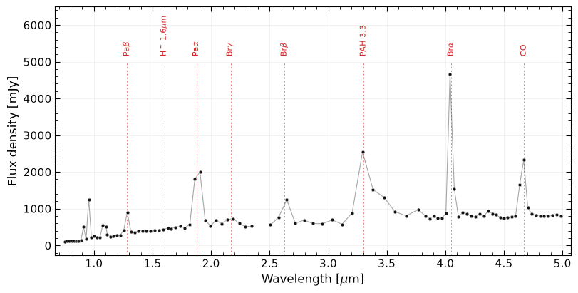
6.4 Show Spectrum in Firefly
Finally, we can also show the spectrum in Firefly directly. The Firefly visualizer even allows to add certain emission lines ones the redshift is fixed. Before doing that, we have to convert our table phot_table in the correct format.
To this end, we define a small function that does the conversion.
def to_spectrum_votable(tbl, wave_col, flux_col, flux_err_col=None):
    '''Serialize a Table as a Spectrum DM VOTable that Firefly recognizes.'''
    utypes = {wave_col: "spec:Spectrum.Data.SpectralAxis.Value",
              flux_col: "spec:Spectrum.Data.FluxAxis.Value"}
    if flux_err_col:
        utypes[flux_err_col] = "spec:Spectrum.Data.FluxAxis.Accuracy.StatError"

    vot = from_table(tbl)
    vt = vot.get_first_table()
    vt.utype = "spec:Spectrum"
    grp = Group(vt)
    for col, utype in utypes.items():
        f = vt.get_field_by_id_or_name(col)
        f.ID, f.utype = col, utype
        grp.entries.append(FieldRef(vt, ref=col))
    vt.groups.append(grp)
    stream = io.BytesIO()
    vot.to_xml(stream)
    return stream
Before we convert the table, we convert mJy to Jy since Firefly does not recognize it as flux unit.
Now we add a new Firefly instance to plot the spectrum, we call it fc_spec.
fc_spec = FireflyClient.make_client(url="https://irsa.ipac.caltech.edu/irsaviewer")And finally, we can load the spectrum.
fc_spec.show_table(file_input=phot_table_firefly,
              tbl_id="spherex-spectrum", title="SPHEREx quick-look spectrum")
{'success': True}Acknowledgements
About this notebook
Updated: 4 November 2026
Contact: Contact IRSA Helpdesk with questions or problems.
Runtime: This notebook takes about 1-3 minutes to run to completion on a machine with 16GB RAM and 4 CPU. Note that the run time depends mostly on your internet connection, as the FITS cube (~300 MB) has to be downloaded by astropy.io.fits.