1. Learning Goals
Open a SPHEREx mosaic cube from the IRSA Mosaic Tool and assign wavelengths to its planes
Measure a quick-view spectrum throught the cube using
PhotUtilsincluding background subtraction.Create a PAH emission line map from a plane in the cube.
Obtain the corresponding GALEX FUV image from IRSA and overlay the PAH map.
2. SPHEREx Overview
SPHEREx is a NASA Astrophysics Medium Explorer mission that launched in March 2025. During its planned two-year mission, SPHEREx will obtain 0.75-5 micron spectroscopy over the entire sky, with deeper data in the SPHEREx Deep Fields. SPHEREx data will be used to:
constrain the physics of inflation by measuring its imprints on the three-dimensional large-scale distribution of matter,
trace the history of galactic light production through a deep multi-band measurement of large-scale clustering,
investigate the abundance and composition of water and biogenic ices in the early phases of star and planetary disk formation.
The community will also mine SPHEREx data and combine it with synergistic data sets to address a variety of additional topics in astrophysics.
More information is available in the SPHEREx Explanatory Supplement.
3. Imports
The following packages must be installed to run this notebook.
# Uncomment the next line to install dependencies if needed.
# !pip install astropy matplotlib numpy photutils reproject astroquery
import copy
import numpy as np
from astropy.io import fits
from astropy.table import Table, vstack, hstack
from astropy.stats import sigma_clipped_stats, SigmaClip
from astropy.wcs import WCS
from astropy.coordinates import SkyCoord
from astropy.nddata import Cutout2D
import astropy.units as u
from photutils.aperture import CircularAperture, CircularAnnulus, ApertureStats, aperture_photometry
from astroquery.ipac.irsa import Irsa
from reproject import reproject_exact
import matplotlib.pyplot as plt
import matplotlib as mpl/home/runner/work/irsa-tutorials/irsa-tutorials/.tox/py312-buildhtml/lib/python3.12/site-packages/tqdm/auto.py:21: TqdmWarning: IProgress not found. Please update jupyter and ipywidgets. See https://ipywidgets.readthedocs.io/en/stable/user_install.html
from .autonotebook import tqdm as notebook_tqdm
Notebook Cell
## Define some plotting formats
def load_plotting_defaults():
    mpl.rcParams['xtick.minor.visible'] = True
    mpl.rcParams['ytick.minor.visible'] = True
    mpl.rcParams['xtick.minor.top'] = True
    mpl.rcParams['xtick.minor.bottom'] = True
    mpl.rcParams['ytick.minor.left'] = True
    mpl.rcParams['ytick.minor.right'] = True
    mpl.rcParams['xtick.major.size'] = 5
    mpl.rcParams['ytick.major.size'] = 5
    mpl.rcParams['xtick.minor.size'] = 3
    mpl.rcParams['ytick.minor.size'] = 3
    mpl.rcParams['xtick.direction'] = 'in'
    mpl.rcParams['ytick.direction'] = 'in'
    mpl.rcParams['xtick.top'] = True
    mpl.rcParams['ytick.right'] = True

load_plotting_defaults()
def_cols = plt.rcParams['axes.prop_cycle'].by_key()['color']
4. Open SPHEREx Mosaic Cube
We first show how to open the SPHEREx mosaic cube and how to assign wavelengths to the different planes in the cube.
The mosaic cube was obtained from the IRSA SPHEREx mosaic tool GUI. The mosaic tool computes a cube (x,y,) from SPHEREx data at a given sky position provided by the user. In brief, the tool gathers all the SPHEREx spectral images at that position, extracts the pixels at similar wavelenghts, and reprojects them into cube layers at the respective wavelengths. The final cube has 102 wavelength layers from 0.75 to . The user can also specify the spatial size of the cube.
Because the IRSA SPHEREx mosaic tool does not have an API, we have created and downloaded the mosaic already and added it to the ./data/ directory.
We first define the path to the mosaic cube.
fn_spherex = "https://irsa.ipac.caltech.edu/data/demos/notebooks/spherex/M101_irsa.fits"Next, we open the image and convert the flux units from MJy/sr to mJy:
We also update the BUNIT keyword in the header to reflect this change.
The cube’s WCS describes three axes — right ascension, declination, and wavelength. For spatial operations like plotting and reprojection we only need the two sky axes, which we extract with WCS.celestial.
We can now open the cube:
with fits.open(fn_spherex) as hdul:
    hdul.info()

    # load wavelength table
    wave_tab_tmp = Table( hdul['WCS-WAVE'].data )

    # Load header
    cube_hdr = hdul["IMAGE"].header

    # calculate pixel scale
    pixscale_mosaic = np.abs(cube_hdr["CDELT1"]*3600) # pixel scale in arcsec/px

    # adjust image units and update header BUNIT
    cube_img = hdul["IMAGE"].data * 23.5045 * (pixscale_mosaic)**2 / 1e3 # Mjy/sr -> mjy
    cube_hdr['BUNIT'] = "mjy"

    # extract the 2D spatial WCS (dropping the spectral axis)
    cube_wcs = WCS(cube_hdr, fobj=hdul).celestial
    print(f"Loaded SPHEREx cube with pixel scale {pixscale_mosaic} arcsec/px")
Filename: /home/runner/.cache/astropy/download/url/fe849a8d38ed3375365307e9e9222675/contents
No. Name Ver Type Cards Dimensions Format
0 PRIMARY 1 PrimaryHDU 5 ()
1 IMAGE 1 ImageHDU 51 (267, 267, 102) float32
2 NHITS 1 ImageHDU 51 (267, 267, 102) int32
3 FLAGS 1 ImageHDU 55 (267, 267, 102) int32
4 SPECTRAL_CHANNELS 1 BinTableHDU 29 102R x 8C [I, I, E, E, E, E, E, E]
5 WCS-WAVE 1 BinTableHDU 18 1R x 3C [102J, 102E, 102E]
Loaded SPHEREx cube with pixel scale 9.0 arcsec/px
WARNING: FITSFixedWarning: The WCS transformation has more axes (4) than the image it is associated with (3) [astropy.wcs.wcs]
Note that the FITS has different layers.
The
IMAGElayer is the actual cube where the 3 dimensions are (x, y, wavelength).The
NHITSlayer includes the number of images that were combined in the mosaic for each pixel.The
FLAGSlayer includes some useful flags to identify outlier and overflow pixels.The
SPECTRAL_CHANNELSlayer summarizes some useful additional information on the spectral channels used to create the cube planes in a binary table.The
WCS-WAVElayer contains a binary table summarizing the wavelength information for each plane in the cube.
5. Create a Quick Look Spectrum
Once we have the cube loaded, let’s generate a quick-look spectrum. This has two purposes: First, it shows how to extract a spectrum from a cube using the PhotUtils python package. Second, it allows us to visualize the wavelength channels (i.e., planes) which we will need to chose the planes to make the final PAH map.
5.1 Create a Wavelength Look-Up Table
Later we will measure an aperture flux on each plane (representing a different wavelength) of the mosaic cube. In order to turn this aperture flux table into a spectrum, we need to track the relevant wavelength range of each plane. Furthermore, the wavelength look-up table will be used to construct the emission line map.
We construct the wavelenght look-up table from the WCS-WAVE layer, which summarizes the wavelength information.
wave_tab = Table( [wave_tab_tmp["PLANE"][0],
                  np.asarray([ww[0] for ww in wave_tab_tmp["WAVELENGTHS"][0] ]),
                  np.asarray([ww[0] for ww in wave_tab_tmp["BANDWIDTHS"][0] ])],
                  names=["plane","wavelengths","bandwidths"],
                dtype=[int, float, float])
Let’s have a look at this table. The bandwidths correspond to the width of each wavelength channel.
wave_tab5.2 Extract Spectrum
To obtain the spectrum, we create a function that computes the sum of the fluxes in apertures and does a background subtraction using an annulus. Both aperture and annulus sizes are user-defined. We use the PhotUtils package for this (see here for more information).
The measurements are done for each cube plane and the combined.
Furthermore, the function creates a plot showing the collapsed cube and the apertures used (this output can be turned off).
Notebook Cell
def measure_aperture_photometry_cube(cube, *, r_aperture_px=20, r_inner_px=60, r_outer_px=100, makeplot=True):
    '''
    Create quick look spectrum from simple aperture photometry with background subtraction
    from annulus.

    Parameters
    ----------
    cube : numpy.ndarray
        Input SPHEREx mosaic cube.
    r_aperture_px : float
        Aperture for flux extraction in pixels.
    r_inner_px : float
        Inner annulus bound for background calculation in pixels.
    r_outer_px : float
        Outer annulus bound for background calculation in pixels.
    MAKEPLOT : book
        Set to `True` if function should create a figure showing the collapsed
        cube with overlay of aperture and annulli.

    Return
    -------
    astropy.QTable
        A table including the photometry results (sum of aperture flux, plane ID, etc).

    '''

    ## Define helper function to compute the photometry efficiently
    def apphot_helper(img , position, aperture, annulus_aperture):
        '''
        Helper function which computes the photometry for a single image.
        Helper function will be called in series to obtain photometry for all images/planes.

        Parameters
        ----------
        img : numpy.ndarray
            Two-dimensional image on which aperture photometry is performed.
        position : tuple of float
            Center position of the aperture.
        aperture : photutils.CircularAperture
            Aperture for photometry extraction.
        annulus_aperture : photutils.CircularAnnulus
            Annulus aperture for background estimation.

        Returns
        -------
        astropy.QTable
            A table including the photometry results (sum of aperture flux, plane ID, etc).

        '''

        ## Calculate background
        sigclip = SigmaClip(sigma=3.0, maxiters=10)
        aperstats = ApertureStats(img, annulus_aperture, sigma_clip=sigclip)
        bkg_mean = aperstats.mean
        aperture_area = aperture.area_overlap(img)
        total_bkg = bkg_mean * aperture_area

        ## Get photometry and subtract background
        phot_table = aperture_photometry(img, aperture)
        phot_table["aperture_sum_bkgsub"] = phot_table["aperture_sum"] - total_bkg

        return(phot_table)


    ## Define position and apertures
    position = (cube.shape[1]//2,cube.shape[2]//2)
    aperture = CircularAperture(position, r=r_aperture_px)
    annulus_aperture = CircularAnnulus(position, r_in=r_inner_px, r_out=r_outer_px)


    ## Compute photometry (use helper function to iterate over planes)
    phot_all = vstack( [apphot_helper(cube[ii,:,:] , position, aperture, annulus_aperture) for ii in range(cube.shape[0])] ) # run all planes
    phot_all["id"] = np.arange(cube.shape[0])+1 ## add plane numbers back
    phot_all.rename_column("id","plane")

    ## Plot if asked for
    if makeplot:

        fig = plt.figure(figsize=(5,5))
        ax1 = fig.add_subplot(1,1,1)

        # Plot the median image:
        img_plot = np.nanmedian(cube, axis=0)
        lims = np.nanpercentile(img_plot.flatten() , q=(5,99.9))
        ax1.imshow(img_plot, origin="lower", vmin=lims[0], vmax=lims[1] , norm="log", cmap="inferno")

        # Plot the center
        ax1.plot(cube.shape[1]//2 , cube.shape[2]//2 , "+" , color="white")

        # plot the apertures
        aperture.plot(ax=ax1 , linestyle="-", color="white", label="Aperture")
        annulus_aperture.plot(ax=ax1 , linestyle=":", color="white", label="Background")

        ax1.legend(loc="lower right", fontsize=9, framealpha = 1, facecolor="black", labelcolor="white")

        ax1.tick_params(which="both", axis="both", color="white", labelsize=11)

        ax1.set_xlabel(r"$x$ [px]")
        ax1.set_ylabel(r"$y$ [px]")

        plt.show()

    return(phot_all)
phot_table = measure_aperture_photometry_cube(cube = cube_img , r_aperture_px = 20, r_inner_px = 60, r_outer_px= 100, makeplot = True)
phot_tableWARNING: MergeConflictWarning: Cannot merge meta key 'date' types <class 'str'> and <class 'str'>, choosing date='2026-09-22 10:54:32 UTC' [astropy.utils.metadata.merge]
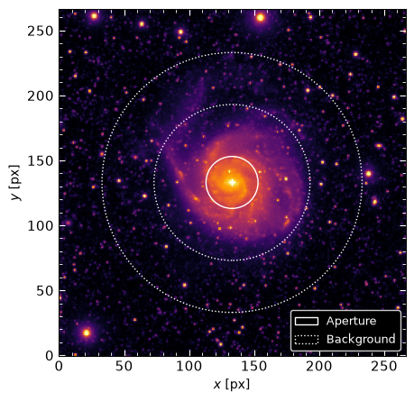
Finally, we also add the wavelength from the wavelength look-up table that created above to the photometry table. This makes it easy to plot the spectrum afterwards.
phot_table["wavelengths"] = wave_tab["wavelengths"].copy()Now that we have all the information, we can plot the spectrum. We also mark some prominent near-infrared emission features for reference.
## Plot Spectrum
fig = plt.figure(figsize=(7,4))
ax1 = fig.add_subplot(1,1,1)

# spectrum
ax1.plot(phot_table["wavelengths"] , phot_table["aperture_sum_bkgsub"], "o", markersize=3, markerfacecolor="black", markeredgecolor="black")

# label emission lines directly on the plot
lines = [
    (1.28, r"Pa-$\beta$"),
    (1.60, r"1.6 $\mu$m bump"),
    (1.87, r"Pa-$\alpha$"),
    (2.36, r"Br-$\beta$"),
    (3.30, r"PAH 3.3 $\mu$m"),
    (4.05, r"Br-$\alpha$"),
]

# plot spectrum and emission lines
trans = mpl.transforms.blended_transform_factory(ax1.transData, ax1.transAxes)
for wave, label in lines:
    ax1.axvline(wave, ymin=0.3, linestyle=":", color="gray", linewidth=0.5)
    ax1.text(wave, 0.05, label, transform=trans, fontsize=7,
             va="bottom", ha="center", rotation=90, color="gray")

ax1.tick_params(which="both", axis="both", labelsize=12)
ax1.set_xlabel(r"Wavelength [$\mu$m]", fontsize=12)
ax1.set_ylabel(r"Flux [mJy]", fontsize=12)

plt.show()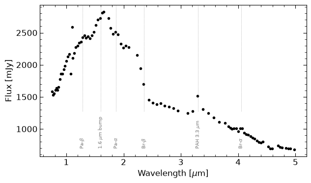
6. Create a PAH Map
We now create the PAH map from the cube. The emission line map is created by subtracting the median of nearby continuum planes from the feature plane.
We first identify the relevant planes by matching the observed PAH wavelength to the entries in wave_tab. For M101 the redshift is negligible, but the same code works for any target — just set z to the known redshift.
z = 0.0  # redshift of target
pah_obs = 3.3 * (1 + z)  # observed PAH wavelength in microns

pah_idx = np.argmin(np.abs(wave_tab["wavelengths"] - pah_obs))
planes_feature = [wave_tab["plane"][pah_idx]]
planes_continuum = list(wave_tab["plane"][[pah_idx - 2, pah_idx - 1, pah_idx + 1, pah_idx + 2]])
print(f"Feature plane: {planes_feature}  ({wave_tab['wavelengths'][pah_idx]:.3f} μm)")
print(f"Continuum planes: {planes_continuum}")
Feature plane: [np.int64(63)] (3.293 μm)
Continuum planes: [np.int64(61), np.int64(62), np.int64(64), np.int64(65)]
We can also visualize the chosen planes on the spectrum plot to for additional checking.
## Plot Spectrum (again, for checking planes)
fig = plt.figure(figsize=(7,4))
ax1 = fig.add_subplot(1,1,1)

# spectrum
ax1.plot(phot_table["wavelengths"] , phot_table["aperture_sum_bkgsub"], "o", markersize=3, markerfacecolor="black", markeredgecolor="black")

# plot spectrum and emission lines
trans = mpl.transforms.blended_transform_factory(ax1.transData, ax1.transAxes)
for wave, label in lines:
    ax1.axvline(wave, linestyle=":", color="gray", linewidth=0.5)
    ax1.text(wave, 0.05, label, transform=trans, fontsize=7,
             va="bottom", ha="center", rotation=90, color="gray")

# indicated planes
[ax1.text(phot_table["wavelengths"][ss-1] , phot_table["aperture_sum_bkgsub"][ss-1]*1.1, phot_table["plane"][ss-1] , fontsize=7, va="bottom", ha="center", rotation=90, color="blue") for ss in planes_feature]
[ax1.text(phot_table["wavelengths"][ss-1] , phot_table["aperture_sum_bkgsub"][ss-1]*1.1, phot_table["plane"][ss-1] , fontsize=7, va="bottom", ha="center", rotation=90, color="red") for ss in planes_continuum]
ax1.plot(phot_table["wavelengths"][np.asarray(planes_feature)-1] , phot_table["aperture_sum_bkgsub"][np.asarray(planes_feature)-1], "o", markersize=3, markerfacecolor="blue", markeredgecolor="blue")
ax1.plot(phot_table["wavelengths"][np.asarray(planes_continuum)-1] , phot_table["aperture_sum_bkgsub"][np.asarray(planes_continuum)-1], "o", markersize=3, markerfacecolor="red", markeredgecolor="red")

ax1.tick_params(which="both", axis="both", labelsize=12)
ax1.set_xlabel(r"Wavelength [$\mu$m]", fontsize=12)
ax1.set_ylabel(r"Flux [mJy]", fontsize=12)

plt.show()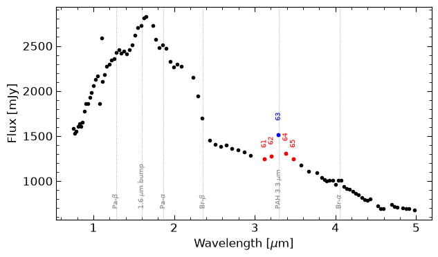
For the map creation, we set up a handy function:
def make_map(cube,
             planes_feature = [63],
             planes_continuum = [61,62,64,65]
            ):
    '''
    Create SPHEREX map from planes. Note that the plane IDs are 1-indexed.

    Parameters
    ----------
    cube : numpy.ndarray
        SPHEREx Mosaic cube.
    planes_feature : list of int
        The cube planes including the emission line feature.
    planes_continuum : list of int
        The cube planes including the continuum which will be subtracted.

    Returns
    -------
    numpy.ndarray
        Two-dimensional map.

    '''
    img_map = np.nansum( cube[np.asarray(planes_feature)-1 , :,:], axis=0 ) - np.nanmedian( cube[np.asarray(planes_continuum)-1 , :,:], axis=0 )
    return(img_map)
With the planes identified, we can now build the map:
img_map = make_map(cube_img, planes_feature=planes_feature, planes_continuum=planes_continuum)Finally, we can plot our PAH SPHEREx map!
fig = plt.figure(figsize=(5,5))
ax1 = fig.add_subplot(1,1,1)
lims = np.nanpercentile(img_map.flatten() , q=(5,99.5))
ax1.imshow(img_map , origin="lower", vmin=lims[0], vmax=lims[1], norm="linear", cmap="inferno")
ax1.tick_params(which="both", axis="both", color="white", labelsize=11)
ax1.set_xlabel(r"$x$ [px]")
ax1.set_ylabel(r"$y$ [px]")
plt.show()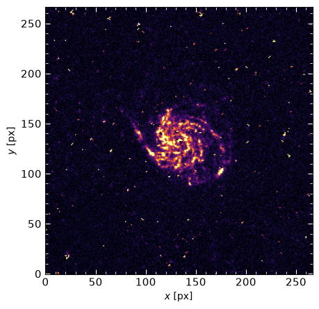
The map shows the location of the PAH emission in the local galaxy M101. Specifically, the feature is an observational indicator of very small carbonageous dust grains. You can see that the PAH emission is not continuous as it is tied to regions of star formation. To explore this further, we can correlate the PAH map with the GALEX far-UV (FUV) continuum map, which maps the UV emission of hot, young stars. This is done in the next section.
7. Get Corresponding GALEX Image
Next we retrieve the GALEX image corresponding to the SPHEREx mosaic. This is scientifically interesting as we can observe how the PAH emission correlates with UV emission of hot young stars. It is expected that there is an anticorrelation as the small PAH grain (traced by the feature) are being dissociated in strong UV radiation fields.
We first obtain the position in coordinates at the center of the SPHEREx cube. Note that this is a 3d cube, so we have to take axes 1 and 2 (0-indexed) to obtain the coordinates!
radec = cube_wcs.all_pix2world(cube_img.shape[2]//2 , cube_img.shape[1]//2 , 0)
print(f"Sky position at R.A. = {radec[0]} and Decl. = {radec[1]}")
pos = SkyCoord(ra=radec[0], dec=radec[1], unit='deg')
Sky position at R.A. = 210.8022671 and Decl. = 54.34895
We then query IRSA at this position to obtain the GALEX FUV image. This data product is part of the Spitzer Local Volume Legacy Survey, which observes many local galaxies. Accordingly, we query the collection spitzer_lvl and search for science images from GALEX in the FUV energy passband.
im_table = Irsa.query_sia(pos=(pos, 1 * u.arcsec), collection='spitzer_lvl')
sel = np.where((im_table["dataproduct_subtype"] == "science") & (im_table["instrument_name"] == "GALEX") & (im_table["energy_bandpassname"] == "FUV") )[0]
im_table[sel]Once we have the table, we can access the URL of the image in the access_url column. With the URL we can load the FITS image and create a cutout of similar size as the SPHEREx mosaic.
image_url = im_table['access_url'][sel][0]
size = u.Quantity([40,40], u.arcmin)

with fits.open(image_url, memmap=False) as hdul:
    hdul.info()
    galex_cutout = Cutout2D(hdul[0].data , position=pos , size=size, wcs = WCS(hdul[0].header), mode="partial")
    img_galex = galex_cutout.data
    wcs_galex = galex_cutout.wcs
    hdr_galex = hdul[0].header
    hdr_galex.update(wcs_galex.to_header()) # update header to cutout.
    hdr_galex["NAXIS1"] = img_galex.shape[1] # update header to cutout.
    hdr_galex["NAXIS2"] = img_galex.shape[0] # update header to cutout.
Filename: /home/runner/.cache/astropy/download/url/adfbacbc3e38c3f9b2d2159447c2aeb7/contents
No. Name Ver Type Cards Dimensions Format
0 PRIMARY 1 PrimaryHDU 137 (3840, 3840) float32
Additionally, we do some post-processing on the image to convert the pixel units to milli-Jansky, similar as the SPHEREx mosaic. Note that the zero points for the GALEX FUV and NUV images are different as defined above. We refer to the Spitzer LVL documentation for more details on the GALEX pixel units.
zps = {"fuv":18.82, "nuv":20.08}
img_galex_ab = -2.5*np.log10(img_galex) + zps["fuv"]
img_galex = 10**(-0.4*(img_galex_ab - 23.9)) / 1e3 # AB -> ujy -> mjy
/tmp/ipykernel_4097/3849881548.py:2: RuntimeWarning: divide by zero encountered in log10
img_galex_ab = -2.5*np.log10(img_galex) + zps["fuv"]
In a last step, we will have to reproject the GALEX image to the SPHEREx mosaic. This is necesary so we can overlap the GALEX image with the PAH map that we have created above. For this, we use the reproject package.
img_galex_rep, fp = reproject_exact(input_data = (img_galex , hdr_galex), output_projection = cube_wcs )
img_galex_rep[img_galex_rep == 0] = np.nan
img_galex_rep = img_galex_rep / np.nansum(img_galex_rep) * np.nansum(img_galex)
Finally, we caon overlay the PAH emission on the GALEX map, which is our final result of this tutorial notebook.
fig = plt.figure(figsize=(9,9))
ax1 = fig.add_subplot(1,1,1)

## Main figure -------

# plot PAH map
lims = np.nanpercentile(img_galex_rep.flatten() , q=(5,99.5))
ax1.imshow(img_galex_rep , origin="lower", vmin=lims[0], vmax=lims[1], norm="linear", cmap="Blues")

# Overplot contours
ax1.contour(img_map, levels=[0.3,0.4,0.5], colors="red", linewidths=0.5)

ax1.set_xlabel(r"$x$ [px]")
ax1.set_ylabel(r"$y$ [px]")


## Inset (zoom-in) -----
axins = ax1.inset_axes([0.5,0.05,0.5,0.3])

center = [125, 120] # center in pixels
width = [70,50] # with in pixels
img_galex_rep_zoom = img_galex_rep[int(center[1]-width[1]/2):int(center[1]+width[1]/2) , int(center[0]-width[0]/2):int(center[0]+width[0]/2)]
img_map_zoom = img_map[int(center[1]-width[1]/2):int(center[1]+width[1]/2) , int(center[0]-width[0]/2):int(center[0]+width[0]/2)]

# plot PAH map
axins.imshow(img_galex_rep_zoom , origin="lower", vmin=lims[0], vmax=lims[1], norm="linear", cmap="Blues")

# Overplot contours
axins.contour(img_map_zoom, levels=[0.3,0.4,0.5], colors="red", linewidths=1)

plt.show()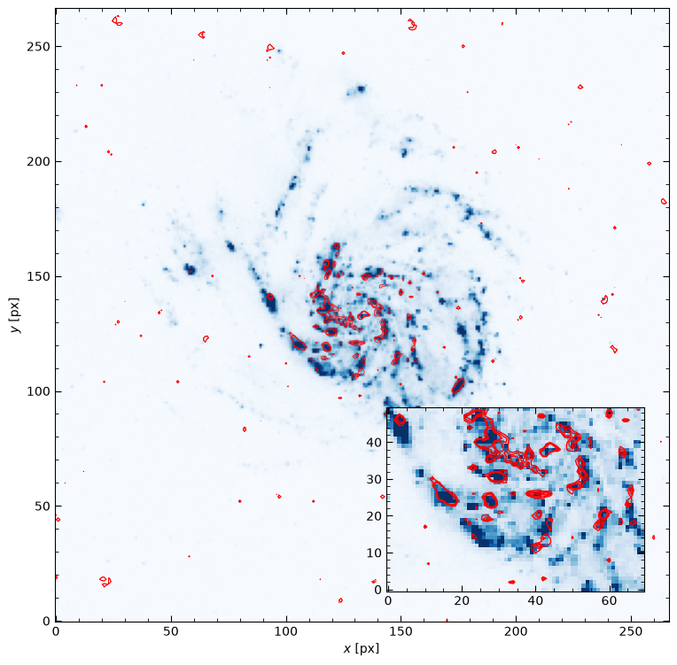
The figure shows the PAH emission (red contours) on top of the GALEX FUV continuum emission (blue). The inset shows a zoom in on the central regions. This comparison confirms that the PAH emission generally follows the location of young hot stars. However, there are also differences (see zoom-in) where there are bright UV regions devoid of PAH emission. This may be the case where the strong ionization fields of young stars dissolve the small dust grains.
Acknowledgements
About this notebook
Updated: 8 May 2026
Contact: Contact IRSA Helpdesk with questions or problems.
Runtime: This notebook takes about 20 seconds to run to completion on a machine with 32GB RAM and 8 CPU.