Learning Goals
By the end of this tutorial, you will be able to:
Browse the OpenUniverse2024 data directories on S3
Explore the structure of Roman and Rubin FITS image files
Read the OpenUniverse2024 parquet catalogs (transient, galaxy, and galaxy flux)
Query Roman and Rubin images covering a sky position using the IRSA SIA service
Introduction
The OpenUniverse2024 simulation suite delivers ~70 deg² of matched optical/infrared imagery for both the LSST Wide-Fast-Deep (WFD) and the Nancy Grace Roman Space Telescope high-latitude survey, producing roughly 400 TB of publicly available synthetic imaging and catalogs. All data are stored in the cloud (AWS S3) and can be accessed anonymously without any credentials.
This tutorial is a focused introduction to data access only. It covers the three main categories:
Directory structure for FITS images — Roman and Rubin simulated science images stored in S3
Parquet catalogs — transient (SNANA), galaxy, and galaxy-flux tables, indexed by HEALPix sky region
Image search via SIA — querying which images cover a given sky position using astroquery and the IRSA Simple Image Access service
No astrophysical analysis is performed here. For science workflows that build on these access patterns, see the TDE Light Curve and SED Fitting tutorials in this repository.
Instructions
This notebook is designed to be run sequentially from top to bottom. All code is self-contained and relies on publicly accessible data.
Input
OpenUniverse2024 Roman and Rubin images and catalogs on AWS S3 (
s3://nasa-irsa-simulations/)
Output
A gallery of example Roman FITS images
Summary of parquet catalog structure and contents
A table of image files overlapping a chosen sky position
Imports
# Uncomment the next line to install dependencies if needed.
# !pip install numpy astropy s3fs photutils matplotlib pyarrow pandas hpgeom astroquery
import numpy as np
import s3fs
from matplotlib import pyplot as plt
import pyarrow.fs
import pyarrow.parquet as pq
import hpgeom
import json
from astroquery.ipac.irsa import Irsa
from astropy.coordinates import SkyCoord
from astropy import units as u
from astropy.io import fits1. Explore Directory Structure for FITS images
The OpenUniverse2024 data live on the cloud in a public AWS S3 bucket and can be accessed anonymously using s3fs. This section shows how to establish that connection, navigate the directory tree, and inspect the contents of a FITS image file.
In the path below, simple_model refers to the simulated images with noise and realistic instrument effects, as opposed to truth images which are noise-free.
The full simulation covers the complete survey footprint. See the OpenUniverse2024 paper for details on how it was produced.
A pointing is a unique Roman observation visit — each pointing corresponds to one placement of the 18-detector focal plane on the sky, producing up to 18 individual FITS files (one per detector).
# Create an anonymous (public read-only) connection to the NASA IRSA S3 bucket.
s3 = s3fs.S3FileSystem(anon=True)

# Top-level path components
BUCKET_NAME = "nasa-irsa-simulations"
OU_PREFIX = "openuniverse2024"
ROMAN_TDS_PREFIX = "roman/full/RomanTDS/images/simple_model"

# Pick one band to explore
BAND = "J129"
band_directory = f"{BUCKET_NAME}/{OU_PREFIX}/{ROMAN_TDS_PREFIX}/{BAND}"
The pointings available for a given band can be listed by calling s3.ls on the band directory.
# List all pointings available for the chosen band
all_pointings = [p.split("/")[-1] for p in s3.ls(band_directory)]
print(f"Found {len(all_pointings)} pointings in band {BAND}:")
print(all_pointings[:10], "...")
Found 8195 pointings in band J129:
['10175', '10176', '10177', '10178', '10179', '10180', '10181', '10182', '10183', '10184'] ...
We pick one of these pointings to explore further.
# Select one pointing and list the files it contains
POINTING = "10190"
image_directory = f"{band_directory}/{POINTING}"

files = [f"s3://{f}" for f in s3.ls(image_directory)]
print(f"Found {len(files)} files in pointing {POINTING}")
Found 18 files in pointing 10190
# Open one FITS file and inspect its extensions
fname = files[0]
with fits.open(fname, use_fsspec=True, fsspec_kwargs={"anon": True}, memmap=False) as hdul:
    print(f"File: {fname}")
    print(f"Number of extensions: {len(hdul)}\n")
    hdul.info()
File: s3://nasa-irsa-simulations/openuniverse2024/roman/full/RomanTDS/images/simple_model/J129/10190/Roman_TDS_simple_model_J129_10190_1.fits.gz
Number of extensions: 4

Filename: <class 's3fs.core.S3File'>
No.    Name      Ver    Type      Cards   Dimensions   Format
  0  PRIMARY       1 PrimaryHDU      63   ()
  1  SCI           1 ImageHDU        68   (4088, 4088)   float64
  2  ERR           1 ImageHDU        68   (4088, 4088)   float32
  3  DQ            1 ImageHDU        70   (4088, 4088)   int32 (rescales to uint32)
Each Roman TDS FITS file contains four extensions: a primary header with no data, followed by three 4088×4088 pixel planes — SCI (science image), ERR (per-pixel uncertainty), and DQ (data quality mask).
Let’s display a gallery of example images to get a sense of the data. Note this gallery can take about a minute to build.
Notebook Cell
def show_gallery(files, max_images=9):
    """
    Display a gallery of FITS images.

    Parameters
    ----------
    files : list of str
        List of S3 URIs to FITS files.
    max_images : int, optional
        Maximum number of images to display (default: 9).
    """
    n_images = min(len(files), max_images)
    ncols = n_images if n_images < 4 else 3
    nrows = (n_images + ncols - 1) // ncols

    fig, axes = plt.subplots(nrows, ncols, figsize=(4 * ncols, 4 * nrows))
    axes = np.atleast_1d(axes).ravel()

    for i, f in enumerate(files[:n_images]):
        with fits.open(f, fsspec_kwargs={"anon": True}, memmap=False) as hdul:
            data = hdul[1].data
            vmin, vmax = np.nanpercentile(data, [5, 99])
            axes[i].imshow(data, origin="lower", cmap="gray", vmin=vmin, vmax=vmax)
            axes[i].set_title(f.split("/")[-1], fontsize=8)
            axes[i].axis("off")

    for j in range(i + 1, len(axes)):
        axes[j].axis("off")

    plt.tight_layout()
    plt.show()
# Display up to 3 images from the selected directory.
show_gallery(files, max_images=3)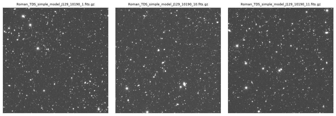
2. Access the Parquet Catalogs
The OpenUniverse2024 catalogs are stored as Apache Parquet files, partitioned by HEALPix sky region (nside=32, RING ordering). Each region has three file types:
snana_{region}.parquet— one row per simulated transient event (supernovae, TDEs, etc.), with event type (model_name) and host galaxy ID (host_id)galaxy_{region}.parquet— host galaxy positions and physical propertiesgalaxy_flux_{region}.parquet— multi-band Roman and Rubin photometry for each galaxy
We first look for the correct catalog for the center of the Roman Time-Domain Survey(TDS). The region number in each filename is the HEALPix pixel index. Because we know that the catalogs were built with nside=32 and RING ordering, we can convert sky coordinates to a region index using hpgeom.
# The Roman Time-Domain Survey is centered near the LSST ELAIS-S1 Deep Drilling Field.
ra = 9.45
dec = -44.02

# Convert sky coordinates to a HEALPix region index (nside=32, RING ordering)
nside = 32
region = hpgeom.angle_to_pixel(nside, ra, dec, lonlat=True, nest=False)
print(f"HEALPix region for RA={ra}, Dec={dec}: {region}")
HEALPix region for RA=9.45, Dec=-44.02: 10307
# Build the S3 paths for this region's catalog files
CATALOG_NAME = "roman_rubin_cats_v1.1.2_faint"
catalog_prefix = f"{BUCKET_NAME}/{OU_PREFIX}/roman/full/{CATALOG_NAME}"

snana_path    = f"{catalog_prefix}/snana_{region}.parquet"
galaxy_path   = f"{catalog_prefix}/galaxy_{region}.parquet"
gal_flux_path = f"{catalog_prefix}/galaxy_flux_{region}.parquet"

print("SNANA file:       ", snana_path)
print("Galaxy info file: ", galaxy_path)
print("Galaxy flux file: ", gal_flux_path)
SNANA file: nasa-irsa-simulations/openuniverse2024/roman/full/roman_rubin_cats_v1.1.2_faint/snana_10307.parquet
Galaxy info file: nasa-irsa-simulations/openuniverse2024/roman/full/roman_rubin_cats_v1.1.2_faint/galaxy_10307.parquet
Galaxy flux file: nasa-irsa-simulations/openuniverse2024/roman/full/roman_rubin_cats_v1.1.2_faint/galaxy_flux_10307.parquet
2.1 Inspect the SNANA Transient Catalog
inspect_parquet_files() reads only the Parquet metadata footer to print the row count and column names — no data is loaded into memory.
We use it here for the SNANA catalog and repeat it for the galaxy info and flux catalogs below.
Notebook Cell
def inspect_parquet_files(s3_path, *, region='us-east-1'):
    """
    Print the structure of a Parquet file on S3 without reading its data.

    Reads only the Parquet metadata footer (row count, column names and types),
    which is fast regardless of file size.

    Parameters
    ----------
    s3_path : str
        S3 path to the Parquet file (without the s3:// prefix).
    """
    fs = pyarrow.fs.S3FileSystem(region=region, anonymous=True)
    meta = pq.read_metadata(s3_path, filesystem=fs)
    schema = pq.read_schema(s3_path, filesystem=fs)

    print(f"Rows: {meta.num_rows}  |  Columns: {len(schema.names)}")
    print("\nColumn names:")
    for name in schema.names:
print(" ", name)inspect_parquet_files(snana_path)Rows: 63151 | Columns: 30
Column names:
id
ra
dec
host_id
gentype
model_name
start_mjd
end_mjd
z_CMB
mw_EBV
mw_extinction_applied
AV
RV
v_pec
host_ra
host_dec
host_mag_g
host_mag_i
host_mag_F
host_sn_sep
peak_mjd
peak_mag_g
peak_mag_i
peak_mag_F
lens_dmu
lens_dmu_applied
model_param_names
model_param_values
MW_av
MW_rv
# Read just the model_name column to see what transient types are in this region
fs = pyarrow.fs.S3FileSystem(region='us-east-1', anonymous=True)
model_names = pq.read_table(snana_path, filesystem=fs, columns=["model_name"]).to_pandas()
model_names["model_name"].unique()
<ArrowStringArray>
[ 'FIXMAG', 'NON1ASED.KN-K17',
'NON1ASED.PISN-STELLA-HECORE', 'NON1ASED.PISN-STELLA-HYDROGENIC',
'NON1ASED.SLSN-I-BBFIT', 'NON1ASED.V19_CC+HostXT_WAVEEXT',
'SALT3.NIR_WAVEEXT', 'NON1ASED.SNIax',
'NON1ASED.TDE-BBFIT']
Length: 9, dtype: str2.2 Inspect the Galaxy Info Catalog
inspect_parquet_files(galaxy_path)Rows: 3561877 | Columns: 18
Column names:
galaxy_id
ra
dec
redshift
redshiftHubble
peculiarVelocity
shear1
shear2
convergence
spheroidHalfLightRadiusArcsec
diskHalfLightRadiusArcsec
diskEllipticity1
diskEllipticity2
spheroidEllipticity1
spheroidEllipticity2
um_source_galaxy_obs_sm
MW_rv
MW_av
2.3 Inspect the Galaxy Flux Catalog
inspect_parquet_files(gal_flux_path)Rows: 3561877 | Columns: 15
Column names:
galaxy_id
lsst_flux_u
lsst_flux_g
lsst_flux_r
lsst_flux_i
lsst_flux_z
lsst_flux_y
roman_flux_W146
roman_flux_R062
roman_flux_Z087
roman_flux_Y106
roman_flux_J129
roman_flux_H158
roman_flux_F184
roman_flux_K213
2.4 Join Transient Events to Their Host Galaxies
A common operation is to take a transient from the SNANA file and look up its host galaxy’s sky position from the galaxy info file.
The two files share a common key: host_id in the SNANA file corresponds to galaxy_id in the galaxy info file.
We read the full SNANA catalog here, then use a filter to fetch only the matching row from the galaxy file without loading the entire galaxy catalog.
Note: The next cell takes ~45s to run
fs = pyarrow.fs.S3FileSystem(region='us-east-1', anonymous=True)

# Read the full SNANA catalog
df_snana = pq.read_table(snana_path, filesystem=fs).to_pandas()

# Pick one transient — here we grab the first row as an example
example_transient = df_snana.iloc[0]
print("Example transient:")
print(example_transient[["model_name", "host_id", "start_mjd", "end_mjd"]])

# Look up its host galaxy by matching host_id (SNANA) to galaxy_id (galaxy info file)
host = pq.read_table(
    galaxy_path,
    filesystem=fs,
    filters=[("galaxy_id", "==", example_transient["host_id"])]
).to_pandas()

print("\nHost galaxy info:")
host
Example transient:
model_name FIXMAG
host_id 10307000149999
start_mjd 63550.0
end_mjd 63570.0
Name: 0, dtype: object
Host galaxy info:
3. Image Search
Given a sky position (e.g., the host galaxy coordinates from Section 2), we can search for all Roman or Rubin images that cover that position using the IRSA Simple Image Access (SIA) service via astroquery.
First we set up the connection to the SIA service and list the available catalogs, then we query by position to get a table of matching images, and finally we extract the cloud locations (S3 URIs) so the files can be opened directly.
# Point the astroquery IRSA client to the correct locations.
Irsa.sia_url = "https://irsa.ipac.caltech.edu/simulated/SIA"
Irsa.tap_url = "https://irsa.ipac.caltech.edu/simulated/TAP"

# List all available simulated image collections
Irsa.list_collections(servicetype='SIA')# Collection names for OpenUniverse2024
OU_ROMAN_SIA_COLLECTION = 'simulated_roman_openuniverse2024'
OU_RUBIN_SIA_COLLECTION = 'simulated_rubin_openuniverse2024'Notebook Cell
def get_s3_fpath(cloud_access):
    """Extract the S3 URI from the cloud_access JSON string in an SIA result."""
    cloud_info = json.loads(cloud_access)
    bucket_name = cloud_info['aws']['bucket_name']
    key = cloud_info['aws']['key']
    return f's3://{bucket_name}/{key}'
# Use the host galaxy position from Section 2 (or set any RA/Dec you want to query).
host_ra = float(host.iloc[0]["ra"])
host_dec = float(host.iloc[0]["dec"])
search_radius = 1 * u.arcsec # small radius: we just need images that contain this point
#convert ra, dec to SkyCoords for ease of use
coords = SkyCoord(host_ra, host_dec, unit='deg')
# Query Roman TDS images in the J129 band
sia_results = Irsa.query_sia(pos=(coords, search_radius.to(u.deg)),
collection=OU_ROMAN_SIA_COLLECTION)
# We first choose to look at the J129 band and the simple_model images
bandname = "J129"
roman_images = sia_results[
['TDS_simple_model' in r['obs_id'] and bandname in r['energy_bandpassname']
for r in sia_results]
]
roman_images['s3_uri'] = [get_s3_fpath(r['cloud_access']) for r in roman_images]
print(f"Found {len(roman_images)} Roman {bandname} images at RA={host_ra:.4f}, Dec={host_dec:.4f}")
roman_images['obs_id', 't_min', 't_max', 's3_uri']Found 176 Roman J129 images at RA=10.9271, Dec=-43.5889
# The same search works for Rubin images — just swap the collection name and band filter.
# Unlike the Roman collection, the Rubin collection contains only one image type (calexp),
# so no obs_id filter is needed beyond selecting the desired band.
rubin_band = "r"
rubin_results = Irsa.query_sia(pos=(coords, search_radius.to(u.deg)),
                               collection=OU_RUBIN_SIA_COLLECTION)

rubin_images = rubin_results[
    [rubin_band in r['energy_bandpassname'] for r in rubin_results]
]
rubin_images['s3_uri'] = [get_s3_fpath(r['cloud_access']) for r in rubin_images]

print(f"Found {len(rubin_images)} Rubin {rubin_band}-band images at RA={host_ra:.4f}, Dec={host_dec:.4f}")
rubin_images['obs_id', 't_min', 't_max', 's3_uri']
Found 2363 Rubin r-band images at RA=10.9271, Dec=-43.5889
You now have S3 URIs for all Roman and Rubin images covering your target position. To open any of these images, pass the URI to astropy.io.fits.open with fsspec_kwargs={"anon": True} as shown in Section 1.
Acknowledgements
This work made use of Astropy:\footnote{http://
www .astropy .org} a community-developed core Python package and an ecosystem of tools and resources for astronomy.
About this notebook
Authors: Jessica Krick, Jaladh Singhal, Brigitta Sipőcz
Updated: 2026-04-22
Contact: IRSA Helpdesk with questions or problems.
Runtime: As of the date above, this notebook takes about 2 minutes to run to completion on a machine with 8GB RAM and 4 CPU.
AI Acknowledgement:
This tutorial was developed with the assistance of AI tools
References:
- Alarcon, A., Aldoroty, L., Beltz-Mohrmann, G., Bera, A., Blazek, J., Bogart, J., Braeunlich, G., Broughton, A., Cao, K., Chiang, J., Chisari, N. E., Desai, V., Fang, Y., Galbany, L., Hearin, A., Heitmann, K., Hirata, C., Hounsell, R., Jain, B., … Zhang, T. (2025). OpenUniverse2024: a shared, simulated view of the sky for the next generation of cosmological surveys. Monthly Notices of the Royal Astronomical Society, 544(4), 3799–3823. 10.1093/mnras/staf1833