Learning Goals
By the end of this tutorial, you will be able to:
access OpenUniverse2024 multiband photometry stored in cloud-based parquet format
plot optical to IR spectral energy distributions(SEDs)
use open-source codes to fit the SED of a sample of targets
Introduction
The OpenUniverse2024 dataset provides simulated multiwavelength observations combining Roman and Rubin realistic survey data. In this tutorial, we walk through a complete technique-focused workflow for analyzing a small sample of galaxies—from accessing the data, to constructing broadband SEDs, to running a first-pass physical model using Prospector.
As an astrophysical case study, we choose to focus on supernova host galaxies. By measuring the SEDs of these hosts across optical to infrared wavelengths, we can estimate key physical properties—such as stellar mass and star formation rate. Comparing these properties between Type Ia and core-collapse supernova hosts helps reveal how different progenitor channels trace galaxy environments. We expect that Type Ia events, originating from older stellar populations, to have occured in more massive, evolved galaxies, whereas we expect core-collapse SNe to follow sites of active star formation in lower-mass systems. Exploring the distribution of supernova type as a function of host stellar mass thus provides direct insight into how stellar evolution, galaxy growth, and transient populations are linked.
Instructions
We use Prospector in this tutorial to do the SED fitting. Running the full SED fitting step in this notebook can take a long time (~30 minutes for a sample of five). You do not need to run those fits unless you want to generate your own results for a custom sample — otherwise. We have provided an output file to explore and visualize the results. If you do want to run the fitting yourself, you will need to uncomment the relevant cell in section 3A.
Input
OpenUniverse 2024 simulated galaxy photometry
OpenUniverse 2024 SN catalogs
In this tutorial, we’ve hard-coded the cloud storage paths for the data files needed to run the examples. This allows you to jump straight into the analysis without worrying about locating or downloading the data manually. If you’d like to learn more about how cloud-based data access works—including how to browse and read files in the cloud—see the IRSA Cloud Access Introduction tutorial.
Output
Plots of SED fits to SN host galaxies
Histogram of SN type as a function host galaxy fitted stellar mass.
Assumptions and Simplifications
In this tutorial we adopt several simplifying assumptions to keep the workflow fast and transparent:
Fixed fractional flux uncertainties (10%) — The OpenUniverse catalogs do not include measurement errors, so we assume a uniform 10 % uncertainty across all bands to allow Prospector to estimate parameter uncertainties.
Rubin to Roman flux scaling — Rubin (LSST) fluxes are rescaled to match Roman normalization at 0.87 µm to correct for small zero-point offsets introduced in the simulations.
Simulated data products — All photometry and supernova catalogs come from the OpenUniverse 2024 simulation; results therefore reflect the assumptions and systematics of the simulated survey, not real observations.
Model choice and priors — Fits use the default Prospector TemplateLibrary[“parametric_sfh”] model with standard priors and an FSPS Chabrier IMF; these settings are meant for demonstration rather than physical tuning.
No explicit dust or attenuation corrections — Aside from what is parameterized within the Prospector model, no additional reddening corrections are applied to the photometry.
Imports
Some dependencies (like fsps and prospector) require specialized setup as described below
import time
starttime = time.time()
# Uncomment to install dependencies if needed.
# %pip install numpy pandas h5py matplotlib seaborn pyarrow gdown
# FSPS + Prospector + SEDPY+ dynasty are required for SED modeling
# If you have trouble installing FSPS, you can skip SED modeling.
# %pip install astro-prospector astro-sedpy "dynesty<2.0.0" fsps pyarrow gdownimport h5py
import pandas as pd
import pyarrow.fs
import pyarrow.parquet as pq
import matplotlib.pyplot as plt
import seaborn as sns
import os
import copy
from multiprocessing import Pool
import numpy as np
import gdown
from sedpy.observate import load_filters, list_available_filters
from prospect.utils.obsutils import fix_obs
from prospect.models.templates import TemplateLibrary
from prospect.sources import CSPSpecBasis
from prospect.plotting import corner1. Define the targets
We begin by identifying our target galaxies — in this example, galaxies hosting simulated supernovae. The OpenUniverse2024 dataset stores different aspects of the data in separate Parquet files:
The SNANA file describes supernova events and their host associations.
The galaxy flux table holds multi-band fluxes from Roman and Rubin.
The galaxy info table includes derived physical parameters (redshift, stellar mass, etc.).
We’ll explore the structure of these Parquet files and then join them into a single table.
1.1 Figure out what is in the OpenUniverse parquet files.
list out some basic information including column names
Notebook Cell
def inspect_parquet_columns(s3_path, *, region='us-east-1', max_rows=0):
    """
    Read Parquet file from S3 into memory and inspect structure

    Parameters
    ----------
    s3_path : str
        Full S3 path to the Parquet file, e.g.
        "s3://nasa-irsa-simulations/openuniverse2024/roman/full/.../SNANA_9921.parquet"
    region : str, optional
        S3 region, default to 'us-east-1' where Fornax is located.
    max_rows : int, optional
        If > 0, print the first few rows of data for context. Default is 0 (just columns).

    Returns
    -------
    pandas.DataFrame
        The full DataFrame loaded from the Parquet file.

    """

    fs = pyarrow.fs.S3FileSystem(region=region, anonymous=True)
    df = pq.read_table(s3_path, filesystem=fs).to_pandas()

    print(f"Found {df.shape[1]} columns and {df.shape[0]} rows")
    print("\nColumn names:")
    for c in df.columns:
        print("  ", c)

    # Optionally, print the first few rows of data for context
    if max_rows > 0:
        print(f"\nFirst {max_rows} rows:")
        print(df.head(max_rows))

    # Return the full DataFrame for further use
    return df
#inspect one of the SN parquet files
sn_flux_file = "nasa-irsa-simulations/openuniverse2024/roman/full/roman_rubin_cats_v1.1.2_faint/snana_9921.parquet"
# These are broken up by region on the sky.
# The region refers to HEALPIX pixel index at nside=32 (order = 5) in the ring numbering scheme
# so in this case the "9921" in the filename refers to that sky region.
df_snana = inspect_parquet_columns(sn_flux_file)
# The output lists number of columns and rows as well as all available column names
# This is useful for exploring what quantities the simulation provides before merging catalogs.Found 30 columns and 5329 rows
Column names:
id
ra
dec
host_id
gentype
model_name
start_mjd
end_mjd
z_CMB
mw_EBV
mw_extinction_applied
AV
RV
v_pec
host_ra
host_dec
host_mag_g
host_mag_i
host_mag_F
host_sn_sep
peak_mjd
peak_mag_g
peak_mag_i
peak_mag_F
lens_dmu
lens_dmu_applied
model_param_names
model_param_values
MW_av
MW_rv
#Now we would like to know what kinds of SN were used in the simulations
#list out the possible SN model names used by OpenUniverse 2024
# See https://arxiv.org/pdf/2501.05632 for a description of these SN models.
df_snana["model_name"].unique()
<ArrowStringArray>
[ 'FIXMAG', 'NON1ASED.PISN-STELLA-HYDROGENIC',
'NON1ASED.SLSN-I-BBFIT', 'NON1ASED.V19_CC+HostXT_WAVEEXT',
'SALT3.NIR_WAVEEXT', 'NON1ASED.SNIax',
'NON1ASED.TDE-BBFIT']
Length: 7, dtype: str1.2 Merge Catalogs
Next we merge the SN sample with the host galaxy fluxes and physical properties. This ensures that each supernova has associated photometric and physical data from its host galaxy, suitable for SED fitting.
Notebook Cell
def assemble_SN_data(sn_flux_file, galaxy_flux_file, galaxy_info_file, *, region='us-east-1'):
    """
    Load a supernova (SNANA) sample and join it with host galaxy flux + info tables.

    Parameters
    ----------
    sn_flux_file : str
        S3 path to the SNANA parquet file, e.g.
        "s3://nasa-irsa-simulations/openuniverse2024/roman/full/.../snana_10050.parquet"
    galaxy_flux_file : str
        S3 path to the galaxy flux parquet (Roman+Rubin flux columns).
    galaxy_info_file : str
        S3 path to the corresponding galaxy info parquet (physical parameters).
    region : str, optional
        S3 region, default to 'us-east-1' where Fornax is located.

    Returns
    -------
    pandas.DataFrame
        Joined DataFrame containing SN + host galaxy properties suitable for SED fitting.
    """

    # Initialize an anonymous (public read-only) S3 filesystem connection
    fs = pyarrow.fs.S3FileSystem(region=region, anonymous=True)

    # Load SN sample
    sn_df = pq.read_table(sn_flux_file, filesystem=fs).to_pandas()
    print(f"  Loaded {len(sn_df)} SN entries")

    # Load galaxy flux and info tables. The flux table is all fluxes and we want
    # every band, but the info table carries a lot of shape and shear columns we
    # never touch, so we ask Parquet for just the three we do use. That leaves
    # about a sixth of the data to pull across and hold in memory.
    gal_flux = pq.read_table(galaxy_flux_file, filesystem=fs).to_pandas()
    gal_info = pq.read_table(
        galaxy_info_file,
        filesystem=fs,
        columns=["galaxy_id", "redshift", "um_source_galaxy_obs_sm"],
    ).to_pandas()

    # Join host-galaxy flux and info tables on galaxy_id
    gal_joined = gal_flux.merge(gal_info, on="galaxy_id", how="inner")
    print(f"  Joined galaxy tables → {len(gal_joined)} rows")

    # Join SN with its host galaxy using host_id
    sn_joined = sn_df.merge(gal_joined, left_on="host_id", right_on="galaxy_id", how="inner")
    print(f"✅ SN–host join completed: {len(sn_joined)} matched hosts")

    # print out the redshift range of the SN sample for reference
    print(f"  Redshift range of SN sample: {sn_joined['z_CMB'].min():.3f}–{sn_joined['z_CMB'].max():.3f}")

    return sn_joined
region = "10050"
sn_flux_file = f"nasa-irsa-simulations/openuniverse2024/roman/full/roman_rubin_cats_v1.1.2_faint/snana_{region}.parquet"
galaxy_flux_file = f"nasa-irsa-simulations/openuniverse2024/roman/full/roman_rubin_cats_v1.1.2_faint/galaxy_flux_{region}.parquet"
galaxy_info_file = f"nasa-irsa-simulations/openuniverse2024/roman/full/roman_rubin_cats_v1.1.2_faint/galaxy_{region}.parquet"
df_sn = assemble_SN_data(sn_flux_file, galaxy_flux_file, galaxy_info_file) Loaded 59584 SN entries
Joined galaxy tables → 3450580 rows
✅ SN–host join completed: 58078 matched hosts
  Redshift range of SN sample: 0.033–2.980
#what does the merged SN dataframe look like?
df_sn#and list out all those column names so we know what we are working with:
print(df_sn.columns.tolist())['id', 'ra', 'dec', 'host_id', 'gentype', 'model_name', 'start_mjd', 'end_mjd', 'z_CMB', 'mw_EBV', 'mw_extinction_applied', 'AV', 'RV', 'v_pec', 'host_ra', 'host_dec', 'host_mag_g', 'host_mag_i', 'host_mag_F', 'host_sn_sep', 'peak_mjd', 'peak_mag_g', 'peak_mag_i', 'peak_mag_F', 'lens_dmu', 'lens_dmu_applied', 'model_param_names', 'model_param_values', 'MW_av', 'MW_rv', 'galaxy_id', 'lsst_flux_u', 'lsst_flux_g', 'lsst_flux_r', 'lsst_flux_i', 'lsst_flux_z', 'lsst_flux_y', 'roman_flux_W146', 'roman_flux_R062', 'roman_flux_Z087', 'roman_flux_Y106', 'roman_flux_J129', 'roman_flux_H158', 'roman_flux_F184', 'roman_flux_K213', 'redshift', 'um_source_galaxy_obs_sm']
1.3 Verify catalog matching worked
To confirm that the SN–host matching worked properly, we compare the supernova redshift (z_CMB) to its host galaxy redshift. A tight correlation along the 1:1 line indicates successful matching.
Notebook Cell
def plot_redshift_comparison(df):
    """
    Plot SN vs. host redshifts to verify consistency

    Parameters
    ----------
    df : pandas.DataFrame
        DataFrame returned by load_SN_data() containing both SN and galaxy columns.

    Returns
    -------
    matplotlib.figure.Figure
        Scatter plot figure comparing z_CMB vs redshift.
    """
    # column names for redshift
    sn_col = "z_CMB"
    gal_col = "redshift"

    # Drop rows with missing or non-finite redshifts
    df_plot = df[[sn_col, gal_col]].dropna()
    df_plot = df_plot[np.isfinite(df_plot[sn_col]) & np.isfinite(df_plot[gal_col])]

    fig, ax = plt.subplots(figsize=(6, 6))
    ax.scatter(df_plot[gal_col], df_plot[sn_col], s=20, alpha=0.6, edgecolor="none")

    # reference line
    zmin = min(df_plot[gal_col].min(), df_plot[sn_col].min())
    zmax = max(df_plot[gal_col].max(), df_plot[sn_col].max())
    ax.plot([zmin, zmax], [zmin, zmax], "r--", lw=1.2, label="1:1 line")

    # Axis labels and aesthetics
    ax.set_xlabel("Galaxy redshift", fontsize=12)
    ax.set_ylabel("SN redshift", fontsize=12)
    ax.set_title("SN vs Host Galaxy Redshift Comparison", fontsize=13)
    ax.legend()

    plt.tight_layout()
    plt.show()
    return
# Plot SN vs. host redshifts to verify consistency
plot_redshift_comparison(df_sn)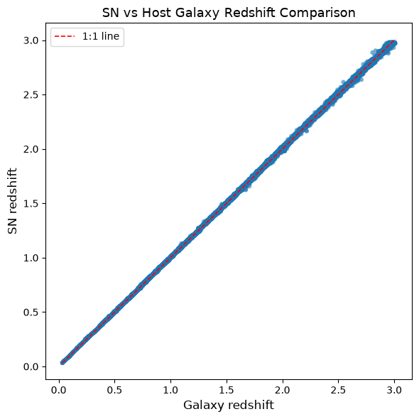
1.4 Save and/or reload the targets
You may want to save your sample of targets to a file and then, next time you need it, skip the cell above and load the sample from file. This can save time when your sample is large, help ensure that the same input data is used for reproduceability, etc.
#filename = "galaxy_sample.csv"

#Save dataframe to .csv
#df_sn.to_csv(filename, index=False)

#reload dataframe from .csv
#df_sn = pd.read_csv(filename)
2. Clean and Visualize data
With the matched sample we just built, we can visualize their spectral energy distributions (SEDs). We will:
Convert photon fluxes into AB maggies using sedpy filter definitions.
Scale Rubin fluxes to match Roman normalization.
Plot SEDs for individual and multiple galaxies.
# Central wavelengths of Rubin and Roman bands in microns
rubin_bands = {
    'lsst_maggies_u': 0.367,
    'lsst_maggies_g': 0.482,
    'lsst_maggies_r': 0.626,
    'lsst_maggies_i': 0.754,
    'lsst_maggies_z': 0.869,
    'lsst_maggies_y': 0.962,
}

roman_bands = {
    'roman_maggies_R062': 0.62,
    'roman_maggies_Z087': 0.87,
    'roman_maggies_Y106': 1.06,
    'roman_maggies_J129': 1.29,
    'roman_maggies_H158': 1.58,
    'roman_maggies_F184': 1.84,
    'roman_maggies_W146': 1.46,
    'roman_maggies_K213': 2.13,
}
Notebook Cell
def scale_rubin_to_roman(df, rubin_bands, roman_bands, match_wave=0.87, verbose=False):
    """
    Scale Rubin (LSST) fluxes so that they match Roman fluxes at a given wavelength.

    This function identifies the Rubin and Roman bands that are closest in wavelength
    to the chosen match point (default = 0.87 µm), computes a per-galaxy scaling factor
    based on their flux ratio, and applies that factor to all Rubin bands so that the
    two instruments are normalized consistently.

    Parameters
    ----------
    df : pandas.DataFrame
        DataFrame containing Rubin and Roman fluxes per galaxy.
        Must include columns like 'lsst_maggies_z' and 'roman_maggies_Z087'.
    rubin_bands : dict
        Mapping of Rubin flux column names to wavelengths (in microns).
        Example: {'lsst_maggies_u': 0.367, 'lsst_maggies_g': 0.482, ...}
    roman_bands : dict
        Mapping of Roman flux column names to wavelengths (in microns).
        Example: {'roman_maggies_Z087': 0.87, 'roman_maggies_H158': 1.58, ...}
    match_wave : float, optional
        Wavelength (in microns) at which the two instruments are scaled to match.
        Default = 0.87 µm (near Roman Z087 / Rubin z band).
    verbose : bool, optional
        If True, print diagnostic info about which bands were matched and the scale factor.

    Returns
    -------
    pandas.DataFrame
        Copy of the input DataFrame, with all Rubin maggie columns rescaled.
    """

    # Make a copy so we don't modify the original DataFrame
    df_scaled = df

    # --- Find Rubin band closest to the target wavelength (match_wave) -------
    smallest_rubin_diff = float("inf")   # Start with a very large difference
    closest_rubin_band = None            # Will hold (band_name, wavelength)

    # Loop through all Rubin bands and measure distance from match_wave
    for band_name, wavelength in rubin_bands.items():

        # Compute how far this band's wavelength is from the target match wavelength
        diff = abs(wavelength - match_wave)

        # If this band is closer than any previous one, store it
        if diff < smallest_rubin_diff:
            smallest_rubin_diff = diff
            closest_rubin_band = (band_name, wavelength)

    # Unpack results: band name and wavelength of the Rubin band closest to match_wave
    rubin_col, rubin_wave = closest_rubin_band

    # --- Find Roman band closest to the target wavelength (match_wave) -------
    smallest_roman_diff = float("inf")   # Start with a very large difference
    closest_roman_band = None            # Will hold (band_name, wavelength)

    # Loop through all Roman bands and measure distance from match_wave
    for band_name, wavelength in roman_bands.items():

        # Compute how far this band's wavelength is from the target match wavelength
        diff = abs(wavelength - match_wave)

        # If this band is closer than any previous one, store it
        if diff < smallest_roman_diff:
            smallest_roman_diff = diff
            closest_roman_band = (band_name, wavelength)

    # Unpack results: band name and wavelength of the Roman band closest to match_wave
    roman_col, roman_wave = closest_roman_band

    # --- Compute the scaling factor (Roman / Rubin) per galaxy ---------------
    scale_factors = df_scaled[roman_col] / df_scaled[rubin_col]

    # --- Optional diagnostic printout if verbose=True ------------------------
    if verbose:
        # Show the matched bands and first few scale factors for verification
        example_factors = scale_factors.head(3).round(3).tolist()
        print(f"Scaling Rubin band {rubin_col} ({rubin_wave:.3f} µm) "
              f"to match Roman band {roman_col} ({roman_wave:.3f} µm)")
        print(f"Example scale factors (Roman/Rubin): {example_factors}")

    # --- Apply the scale factor to all Rubin bands ---------------------------
    for col in rubin_bands.keys():

        #Each Rubin flux is multiplied by its galaxy’s individual scale factor.
        df_scaled[col] = df_scaled[col] * scale_factors

    return df_scaled
Notebook Cell
def photons_to_maggies_with_filter(photon_flux, filt):
    """
    Convert band-integrated photon flux [photons/s/cm^2] to AB maggies,
    using sedpy filter definitions to get effective wavelength and width.

    Parameters
    ----------
    photon_flux : float
        Band-integrated photon flux [photons/s/cm^2].
    filt : sedpy.observate.Filter
        Filter object from sedpy.load_filters (must include wave_effective and width).

    Returns
    -------
    float
        Flux in maggies (AB system).
    """
    h = 6.62607015e-27  # erg s
    c = 2.99792458e18   # Å/s

    lam = filt.wave_effective   # effective wavelength [Å]

    # Effective filter width in Å (integral of throughput)
    delta_lambda = np.trapezoid(filt.transmission, filt.wavelength)

    # photon energy at central wavelength
    E_photon = h * c / lam

    # photon flux integrated over the band → flux density per Å
    f_lambda = (photon_flux * E_photon) / delta_lambda  # erg/s/cm^2/Å

    # convert to f_nu
    f_nu = f_lambda * lam**2 / c

    # AB maggies
    mag_ab = -2.5 * np.log10(f_nu) - 48.6

    #maggies
    maggies = 10**(-0.4 * mag_ab)

    return maggies
Notebook Cell
def add_maggie_columns(df):
    """
    Add maggie flux columns to DataFrame, one per Rubin+Roman band.
    Uses sedpy filter definitions to compute maggies correctly.

    Parameters
    ----------
    df : pandas.DataFrame
        Must contain flux columns (photons/s/cm^2) for Rubin+Roman bands.

    Returns
    -------
    pandas.DataFrame
        Same dataframe with new *_maggies columns.
    """
    # Map catalog flux column names to sedpy filter names
    filter_map = {
        "lsst_flux_u": "lsst_baseline_u",
        "lsst_flux_g": "lsst_baseline_g",
        "lsst_flux_r": "lsst_baseline_r",
        "lsst_flux_i": "lsst_baseline_i",
        "lsst_flux_z": "lsst_baseline_z",
        "lsst_flux_y": "lsst_baseline_y",
        "roman_flux_R062": "roman_wfi_f062",
        "roman_flux_Z087": "roman_wfi_f087",
        "roman_flux_Y106": "roman_wfi_f106",
        "roman_flux_J129": "roman_wfi_f129",
        "roman_flux_W146": "roman_wfi_f146",
        "roman_flux_H158": "roman_wfi_f158",
        "roman_flux_F184": "roman_wfi_f184",
        "roman_flux_K213": "roman_wfi_f213",
    }

    # Load all needed filters once
    filter_names = list(filter_map.values())
    filters = load_filters(filter_names)
    filter_dict = dict(zip(filter_names, filters))

    # Apply conversion
    for col, filt_name in filter_map.items():
        filt = filter_dict[filt_name]
        new_col = col.replace("flux", "maggies")
        df[new_col] = df[col].apply(lambda f: photons_to_maggies_with_filter(f, filt))

    return df
Notebook Cell
def plot_single_sed(df, rubin_bands, roman_bands, galaxy_index=0, loglog=False):
    """
    Plot the Spectral Energy Distribution (SED) for a galaxy in the DataFrame.

    Parameters
    ----------
    df : pandas.DataFrame
        DataFrame containing Rubin and Roman photometric flux columns in units of maggies
        (e.g., 'lsst_maggies_g', 'roman_maggies_F184') and a 'galaxy_id' column.
    rubin_bands : dict
        Mapping of Rubin band names to their central wavelengths in microns.
        Example: {'lsst_maggies_u': 0.367, 'lsst_maggies_g': 0.482, ...}
    roman_bands : dict
        Mapping of Roman band names to their central wavelengths in microns.
        Example: {'roman_maggies_R062': 0.62, 'roman_maggies_Z087': 0.87, ...}
    galaxy_index : int, optional
        Index (integer position) or label of the galaxy row to plot.
        Default is 0 (the first row in the DataFrame).
    loglog : bool, optional
        If True, use logarithmic scaling for both axes. Default is False.

    Returns
    -------
    None
        Displays a matplotlib plot of flux vs. wavelength for the selected galaxy.
    """
    # Select target galaxy row safely (by index or ID)
    try:
        row = df.iloc[galaxy_index]
    except IndexError as e:
        raise ValueError(
            f"Galaxy index {galaxy_index} is out of range for DataFrame "
            f"with {len(df)} rows."
        ) from e

    # Rubin
    rubin_items = sorted(rubin_bands.items(), key=lambda x: x[1])
    rubin_waves = [w for _, w in rubin_items]
    rubin_fluxes = [row[col] for col, _ in rubin_items]


    # Roman
    roman_items = sorted(roman_bands.items(), key=lambda x: x[1])
    roman_waves = [w for _, w in roman_items]
    roman_fluxes = [row[col] for col, _ in roman_items]

    # Plotting
    fig, ax = plt.subplots()

    if loglog:
        ax.set_xscale("log")
        ax.set_yscale("log")

    ax.plot(rubin_waves, rubin_fluxes, marker='o', color='#377eb8', label='Rubin')
    ax.plot(roman_waves, roman_fluxes, marker='o', color='#e41a1c', label='Roman')

    ax.set_xlabel("Wavelength (μm)")
    #ax.set_ylabel("Flux (photons / sec / cm²)")
    ax.set_ylabel("Flux (maggies)")
    galaxy_label = row.get("galaxy_id", galaxy_index)
    ax.set_title(f"SED for Galaxy {galaxy_label}")
    ax.legend()
    plt.tight_layout()
    plt.show()
We now plot flux versus wavelength for one galaxy, comparing Roman and Rubin photometric points. The goal is to get a qualitative sense of the galaxy’s broadband SED shape.
#remove all targets which are not SN
df = df_sn[~df_sn["model_name"].isin(["FIXMAG", "NON1ASED.TDE-BBFIT"])].copy()

# Add maggies to df
df_scaled = add_maggie_columns(df)

# Scale Rubin to Roman
# This is required because the two different instruments do not align in flux in the simulation
df_scaled = scale_rubin_to_roman(df_scaled, rubin_bands, roman_bands)
# Plot an SED
plot_single_sed(df_scaled, rubin_bands, roman_bands, 1, loglog=True)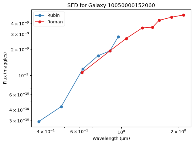
Notebook Cell
def plot_many_seds(df, rubin_bands, roman_bands, n_galaxies=10, loglog=False):
    """
    Plot SEDs for multiple galaxies from the DataFrame.

    Parameters
    ----------
    df : pandas.DataFrame
        DataFrame containing Rubin and Roman flux columns.
    rubin_bands : dict
        Mapping of Rubin band names to their central wavelengths in microns.
        Example: {'lsst_maggies_u': 0.367, 'lsst_maggies_g': 0.482, ...}
    roman_bands : dict
        Mapping of Roman band names to their central wavelengths in microns.
        Example: {'roman_maggies_R062': 0.62, 'roman_maggies_Z087': 0.87, ...}
    n_galaxies : int, optional
        Number of galaxies (rows) to plot. Default is 10.
    loglog : bool, optional
        If True, use log-log scale for both axes. Default is False.

    Returns
    -------
    None
        Displays a matplotlib plot of flux vs. wavelength for multiple galaxies.
    """

    # Rubin bands
    rubin_items = list(rubin_bands.items())
    rubin_cols = [col for col, _ in rubin_items]
    rubin_waves = [wave for _, wave in rubin_items]

    # Roman bands
    roman_items = list(roman_bands.items())
    roman_cols = [col for col, _ in roman_items]
    roman_waves = [wave for _, wave in roman_items]

    fig, ax = plt.subplots()

    if loglog:
        ax.set_xscale("log")
        ax.set_yscale("log")

    for i in range(min(n_galaxies, len(df))):
        rubin_fluxes = df.iloc[i][rubin_cols].to_numpy(dtype=float)
        roman_fluxes = df.iloc[i][roman_cols].to_numpy(dtype=float)

        ax.plot(rubin_waves, rubin_fluxes, marker='o', linestyle='-', color='#377eb8', alpha=0.6)
        ax.plot(roman_waves, roman_fluxes, marker='o', linestyle='-', color='#e41a1c', alpha=0.6)

    ax.set_xlabel("Wavelength (μm)")
    ax.set_ylabel("Flux (maggies)")
    ax.set_title(f"SEDs for {min(n_galaxies, len(df))} Galaxies")
    ax.legend(["Rubin", "Roman"], loc="best")
    plt.tight_layout()
    plt.show()
plot_many_seds(df_scaled, rubin_bands, roman_bands, n_galaxies=50, loglog=True)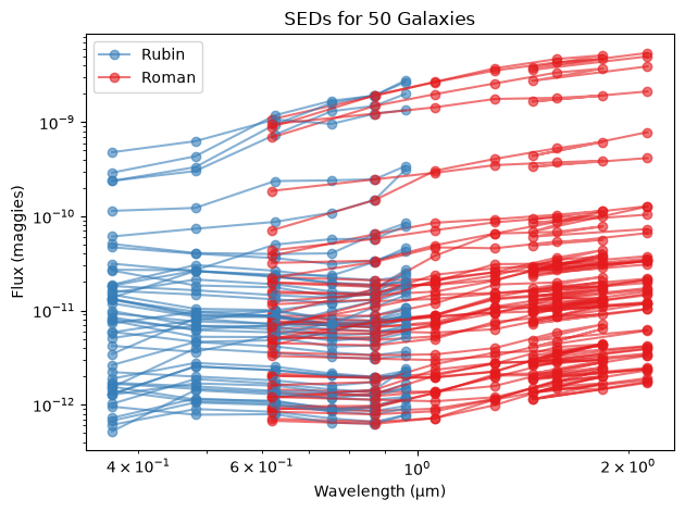
3. SED fitting
In this section we will use Prospector, a Bayesian SED fitting code built on FSPS, to infer stellar population parameters for our galaxies by fitting their SEDs. We choose Prospector because it is an open-source, powerful, yet flexible package to infer stellar population properties that is widely used in the community.
There are two ways to proceed, depending on whether you want to run your own fits or use existing results.
Option A — Run new fits (slow)
This option performs fresh Prospector fits for a small subset of galaxies (20 by default). It is the most transparent path, showing every step of the fitting process and how the models are generated. However, it is computationally expensive — each fit can take several minutes, and the total run may exceed half an hour on a modest machine.
Choose this option if you:
want to learn how Prospector actually performs the fitting,
wish to modify model parameters or fitting settings
Option B — Use existing results(fast)
This option simply reads the saved results (sn_fits.h5) from a previous run.
It is ideal for quickly exploring the fitted parameters, verifying trends, or reproducing plots without waiting for new fits to complete.
Choose this option if you:
are mainly interested in visualizing and analyzing results,
do not need to change the fitting configuration
Both paths produce the same variables — df_small, obs_list, and outputs — so all of the downstream analysis and plotting cells will work identically.
If you are following this notebook for the first time, start with Option B by leaving RUN_FITS = Falseto get a sense of the workflow, and come back later to experiment with Option A when you are ready to explore the full fitting process.
# Leave this as False to load existing galaxy fits
# Change this to True to run Prospector fitting

RUN_FITS = False
3A. Run new SED fits (optional, slow)
Prospector has its own built in functions to do writing and reading, but
they don’t work for multiple galaxy fits, and
they error out on numpy not liking something, so we’ll build our own below called
save_outputs_hdf5
Notebook Cell
def df_to_all_obs(df, flux_err_frac=0.1):
    """
    Convert all galaxies in df into a list of Prospector obs dicts.

    Parameters
    ----------
    df : pandas.DataFrame
        Must contain *_maggies columns (from add_maggie_columns), 'redshift', and 'galaxy_id'.
    flux_err_frac : float
        Fractional flux error to assume.  The OpenUniverse catalogs don't give flux uncertainties
        default is to assume 10% uncertainties in the fluxes.

    Returns
    -------
    list of dict
        Each element is an obs dictionary for one galaxy.
    """
    # Define Rubin and Roman maggie column names
    rubin_maggies = [f"lsst_maggies_{b}" for b in "ugrizy"]
    roman_maggies = ["roman_maggies_R062","roman_maggies_Z087","roman_maggies_Y106",
                     "roman_maggies_J129","roman_maggies_W146","roman_maggies_H158",
                     "roman_maggies_F184","roman_maggies_K213"]

    # Define corresponding sedpy filter names for Rubin and Roman
    rubin_filters = [f"lsst_baseline_{b}" for b in "ugrizy"]
    roman_filters = ["roman_wfi_f062","roman_wfi_f087","roman_wfi_f106",
                     "roman_wfi_f129","roman_wfi_f146","roman_wfi_f158",
                     "roman_wfi_f184","roman_wfi_f213"]
    # Load all sedpy Filter objects at once
    filters = load_filters(rubin_filters + roman_filters)

    obs_list = []

    # Loop over galaxies and build a Prospector obs dict for each
    for _, row in df.iterrows():
        mags = row[rubin_maggies + roman_maggies].to_numpy(dtype=float)
        mags_unc = mags * flux_err_frac
        obs = dict(
            wavelength=None,
            spectrum=None,
            unc=None,
            redshift=row["redshift"],
            maggies=mags,
            maggies_unc=mags_unc,
            filters=filters,
            galaxy_id=int(row["galaxy_id"])  # <-- keep track of galaxy
        )
        obs_list.append(fix_obs(obs))

    return obs_list
Notebook Cell
def process_output(output, model, obs, sps):
    """
    Convert raw output from fit_model into a plotting-ready results dict.
    This stuff all happens as part of prospector's read_results,
    but to avoid IO, we don't use write_results followed by read_results for every galaxy

    Works with both optimization-only and dynesty sampling runs
    in Prospector 1.4 (PyPI release).

    Parameters
    ----------
    output : dict
        Raw dictionary returned by fit_model.
    model : SpecModel
        Prospector model object used in the fit.
    obs : dict
        Observed data dictionary for one galaxy. Must contain 'galaxy_id'.
    sps : CSPSpecBasis
        SPS object used in the fit.

    Returns
    -------
    out_proc : dict
        Results dictionary with at least:
        - 'galaxy_id' : int
        - 'chain' : ndarray
        - 'weights' : ndarray
        - 'theta_labels' : list
        - 'bestfit' : dict with:
            'theta', 'spectrum', 'photometry',
            'restframe_wavelengths',
            'SFR_now', 'SFR_100', 'logSFR_100'
    """
    out_proc = {}

    # Always copy galaxy_id from obs
    out_proc["galaxy_id"] = obs["galaxy_id"]

    # --- case 1: dynesty sampler was run ---
    if output.get("sampling") and output["sampling"][0] is not None:
        # Unpack the dynesty sampler object
        sampler, _ = output["sampling"]

        # Extract posterior samples, weights, and evidence
        chain = sampler.samples
        logwt = sampler.logwt
        logz = sampler.logz[-1]
        weights = np.exp(logwt - logz)

        # Store posterior chain, normalized weights, parameter labels, and log-likelihoods
        out_proc["chain"] = chain
        out_proc["weights"] = weights / np.sum(weights)
        out_proc["theta_labels"] = model.free_params
        out_proc["lnprobability"] = sampler.logl

        # Identify the best-fit sample = max likelihood sample
        imax = np.argmax(sampler.logl)
        theta_best = chain[imax]

        # Predict model spectrum and photometry for the best-fit parameters
        spec, phot, mfrac = model.predict(theta_best, obs=obs, sps=sps)

        # Store best-fit results
        out_proc["bestfit"] = {
            "theta": theta_best,
            "spectrum": spec,
            "photometry": phot,
            "restframe_wavelengths": sps.wavelengths,
        }

    # --- case 2: optimization only ---
    elif output.get("optimization") and output["optimization"][0] is not None:

        # Unpack optimization results and extract best-fit parameters
        opt_result, _ = output["optimization"]
        theta_best = opt_result.x

        # Predict model spectrum and photometry for the optimized parameters
        spec, phot, mfrac = model.predict(theta_best, obs=obs, sps=sps)

        # Store best-fit results in same format as dynesty case
        out_proc["chain"] = np.array([theta_best])
        out_proc["weights"] = np.array([1.0])
        out_proc["theta_labels"] = model.free_params
        out_proc["bestfit"] = {
            "theta": theta_best,
            "spectrum": spec,
            "photometry": phot,
            "restframe_wavelengths": sps.wavelengths,
        }

    else:
        raise ValueError("Output has neither sampling nor optimization results")

    return out_proc
Notebook Cell
def run_fit(obs, model_params, sps, lnprobfn, noise_model, fitting_kwargs):
    """
    Run a single Prospector fit for one galaxy.

    Parameters
    ----------
    obs : dict
        Prospector obs dictionary for one galaxy.
    model_params : dict
        Template dictionary of model parameters (from TemplateLibrary).
        A fresh model will be instantiated for each galaxy.
    sps : prospect.sources.CSPSpecBasis
        FSPS spectral basis (reused across galaxies).
    lnprobfn : callable
        Prospector log-probability function.
    noise_model : optional
        Noise model (usually None).
    fitting_kwargs : dict
        Extra fitting keyword arguments.

    Returns
    -------
    dict
        Output dictionary from fit_model.
    """
    galaxy_id = obs.get("galaxy_id", None)
    print(f"[Galaxy {galaxy_id}] Starting fit...")

    # Make a fresh copy of model params
    model_params = copy.deepcopy(model_params)

    # Initialize redshift per galaxy
    model_params["zred"]["init"] = obs["redshift"]

    # Initialize a Prospector spectral model using the chosen parameter set
    model = SpecModel(model_params)

    # Run the full Prospector fitting routine for this galaxy
    output = fit_model(
        obs,                 # observation dictionary for one galaxy
        model,               # Prospector spectral model (SpecModel instance)
        sps,                 # FSPS stellar population synthesis object
        optimize=False,      # skip optimization-only mode
        dynesty=True,        # use dynesty nested sampling for Bayesian inference
        lnprobfn=lnprobfn,   # log-probability function (likelihood)
        noise=noise_model,   # optional noise model (usually None)
        **fitting_kwargs     # additional sampler settings (e.g., nlive, dlogz)
    )

    # post-processing
    processed = process_output(output, model, obs, sps)

    print(f"[Galaxy {galaxy_id}] Finished fit and post processing.")

    return processed
Notebook Cell
def run_fit_star(args):
    """
    Wrapper function to unpack arguments for ``run_fit`` when using
    ``multiprocessing.Pool.imap_unordered``.

    ``imap_unordered`` passes each element of an iterable as a *single*
    positional argument to the worker function. Since ``run_fit`` expects
    multiple separate arguments (``obs``, ``model_params``, ``sps``,
    ``lnprobfn``, ``noise_model``, ``fitting_kwargs``), this wrapper
    unpacks the input tuple and forwards its contents to ``run_fit``.

    Parameters
    ----------
    args : tuple
        A tuple containing the full set of arguments required by
        ``run_fit`` in the following order:

        ``(obs, model_params, sps, lnprobfn, noise_model, fitting_kwargs)``

    Returns
    -------
    dict
        The processed Prospector output dictionary returned by ``run_fit``.

    Notes
    -----
    This function exists *only* to allow ``run_fit`` to be used with
    ``Pool.imap_unordered``. Unlike ``Pool.starmap``, which unpacks tuples
    automatically but returns results in input order,
    ``imap_unordered`` does not unpack tuples and yields results as soon
    as they are completed, providing better parallel efficiency for fits
    with variable runtimes.

     """
    return run_fit(*args)
Notebook Cell
def fit_sample_parallel(obs_list, model_params, sps, lnprobfn, noise_model=(None,None),
                        fitting_kwargs=None, nproc=None):
    """
    Fit a sample of galaxies in parallel using multiprocessing.

    Parameters
    ----------
    obs_list : list of dict
        List of Prospector obs dictionaries (one per galaxy).
    model_params : dict
        Model parameter dictionary (e.g. TemplateLibrary["parametric_sfh"]).
    sps : prospect.sources.CSPSpecBasis
        FSPS spectral basis (shared).
    lnprobfn : callable
        Prospector log-probability function.
    noise_model : optional
        Noise model (usually (None,None)).
    fitting_kwargs : dict, optional
        Extra kwargs for fit_model.
    nproc : int, optional
        Number of parallel processes.

    Returns
    -------
    raw_results
        List of Prospector output dicts, one per galaxy.
    """
    # determine optimal number of processes = min(#galaxies to fit, available CPU - 1)
    if nproc is None:
        available = os.cpu_count() or 1
        nproc = min(len(obs_list), max(1, available - 1))

    args = [(obs, model_params, sps, lnprobfn, noise_model, fitting_kwargs)
            for obs in obs_list]

    #multiprocessing around run_fit function
    chunksize = max(1, len(args) // (4 * nproc))
    results = []
    with Pool(processes=nproc) as pool:
        for processed in pool.imap_unordered(run_fit_star, args, chunksize=chunksize):
            results.append(processed)

    return results
Notebook Cell
def save_outputs_hdf5(outputs, obs_list, filename="all_galaxies.h5"):
    """
    Save multiple galaxy fit results and corresponding obs dicts to a single HDF5 file.

    Parameters
    ----------
    outputs : list of dict
        Each element is a processed output (from process_output), one per galaxy.
        Must contain 'galaxy_id'.
    obs_list : list of dict
        Each element is an obs dictionary corresponding to the outputs.
        Must contain 'galaxy_id'.
    filename : str, optional
        Output HDF5 filename.
    """
    with h5py.File(filename, "w") as f:
        for out, obs in zip(outputs, obs_list):
            gid = str(out["galaxy_id"])
            # Each galaxy gets its own group named by galaxy_id
            g = f.create_group(gid)

            # ---- save results ----
            g.create_dataset("chain", data=out["chain"])
            g.create_dataset("weights", data=out["weights"])
            g.create_dataset("theta_labels", data=np.array(out["theta_labels"], dtype="S"))

            bestfit_grp = g.create_group("bestfit")
            for k, v in out["bestfit"].items():
                bestfit_grp.create_dataset(k, data=v)

            # ---- save obs ----
            obs_grp = g.create_group("obs")
            obs_grp.create_dataset("redshift", data=obs["redshift"])
            obs_grp.create_dataset("maggies", data=obs["maggies"])
            obs_grp.create_dataset("maggies_unc", data=obs["maggies_unc"])
            filt_names = [f.name for f in obs["filters"]]
            obs_grp.create_dataset("filters", data=np.array(filt_names, dtype="S"))

    print(f"[save] Wrote {len(outputs)} galaxies to {filename}")
3A. Step 1: Explore fitting options
One set of options you have when using Prospector is which filters to use.
OpenUniverse uses Rubin and Roman data but Prospector can include many other filters.
A list of all available sedpy filters are here
or you can list out the available filters below.
print(list_available_filters()[:20]) # peek at first 20['acs_wfc_f435w', 'acs_wfc_f475w', 'acs_wfc_f555w', 'acs_wfc_f606w', 'acs_wfc_f625w', 'acs_wfc_f775w', 'acs_wfc_f814w', 'acs_wfc_f850lp', 'bass_g', 'bass_r', 'bessell_B', 'bessell_I', 'bessell_R', 'bessell_U', 'bessell_V', 'cfht_megacam_gs_9401', 'cfht_megacam_is_9701', 'cfht_megacam_rs_9601', 'cfht_megacam_us_9301', 'cfht_megacam_zs_9801']
A second set of options is which star formation history to choose. Here we show a basic description of all pre-defined parameter sets.
TemplateLibrary.show_contents()'type_defaults':
Explicitly sets dust amd IMF types.
'ssp':
Basic set of (free) parameters for a delta function SFH
'parametric_sfh':
Basic set of (free) parameters for a delay-tau SFH.
'dust_emission':
The set of (fixed) dust emission parameters.
'nebular':
The set of nebular emission parameters, with gas_logz tied to stellar logzsol.
'nebular_marginalization':
Marginalize over emission amplitudes line contained inthe observed spectrum
'fit_eline_redshift':
Fit for the redshift of the emission lines separatelyfrom the stellar redshift
'agn_eline':
Add AGN emission lines
'outlier_model':
The set of outlier (mixture) models for spectroscopy and photometry
'agn':
The set of (fixed) AGN dusty torus emission parameters.
'igm':
The set of (fixed) IGM absorption parameters.
'spectral_smoothing':
Set of parameters for spectal smoothing.
'optimize_speccal':
Set of parameters (most of which are fixed) for optimizing a polynomial calibration vector.
'fit_speccal':
Set of parameters (most of which are free) for sampling the coefficients of a polynomial calibration vector.
'burst_sfh':
The set of (fixed) parameters for an SF burst added to a parameteric SFH, with the burst time controlled by `fage_burst`.
'logm_sfh':
Non-parameteric SFH fitting for log-mass in fixed time bins
'continuity_sfh':
Non-parameteric SFH fitting for mass in fixed time bins with a smoothness prior
'continuity_flex_sfh':
Non-parameteric SFH fitting for mass in flexible time bins with a smoothness prior
'continuity_psb_sfh':
Non-parameteric SFH fitting for mass in Nfixed fixed bins and Nflex flexible time bins with a smoothness prior
'dirichlet_sfh':
Non-parameteric SFH with Dirichlet prior (fractional SFR)
'stochastic_sfh':
Stochastic SFH which correlates the SFRs between time bins based on model in TFC2020
'alpha':
The prospector-alpha model, Leja et al. 2017
'beta':
The prospector-beta model; Wang, Leja, et al. 2023
3A. Step 2: Model setup
# we choose a parametric star formation history model to use for generic galaxy fitting
model_params = TemplateLibrary["parametric_sfh"]

#disable any extra noise modeling and use only the measurement uncertainties provided in the data.
noise_model = (None, None)

fitting_kwargs = dict(
    # Number of live points used by dynesty; higher = better posterior sampling but slower
    nlive_init=800, #200
    # Dynesty sampling strategy; 'rwalk' is robust for multi-dimensional, correlated posteriors.
    nested_method="rwalk",
    # Target number of effective posterior samples before termination; controls fit thoroughness.
    nested_target_n_effective=800, #300
    # Convergence threshold in log-evidence; smaller values force deeper exploration of the posterior.
    nested_dlogz_init=0.05  #0.2
)
3A. Step 3: Data setup
This cell prepares the data for fitting by choosing a small subset of galaxies to fit and putting the data into the format that is expected by Prospector.
# Select a small subset of galaxies to fit

# --- Select 10 SN Ia and 10 Core-Collapse (CC) host galaxies for fitting ---
#increasing this number will increase fitting time

# Identify Type Ia and Core-Collapse SNe by model_name
# OpenUniverse2024 convention: "SALT3.NIR_WAVEEXT" → Type Ia
sn1a = df_scaled[df_scaled["model_name"] == "SALT3.NIR_WAVEEXT"]
ccsn = df_scaled[df_scaled["model_name"] != "SALT3.NIR_WAVEEXT"]

# Randomly sample up to 10 of each (or fewer if limited)
sn1a_sample = sn1a.sample(n=min(10, len(sn1a)), random_state=42)
ccsn_sample = ccsn.sample(n=min(10, len(ccsn)), random_state=42)

# Concatenate
df_small = pd.concat([sn1a_sample, ccsn_sample]).reset_index(drop=True)

print(f"Selected {len(df_small)} host galaxies ({len(sn1a_sample)} Ia + {len(ccsn_sample)} CC)")
print(df_small['model_name'].value_counts())
Selected 20 host galaxies (10 Ia + 10 CC)
model_name
SALT3.NIR_WAVEEXT 10
NON1ASED.V19_CC+HostXT_WAVEEXT 9
NON1ASED.SNIax 1
Name: count, dtype: int64
#Prospector expects a specific obs dictionary format containing fluxes, uncertainties, filters, and redshift.
obs_list = df_to_all_obs(df_small, flux_err_frac=0.1)

# Peek at first galaxy
obs_list[0]
{'wavelength': None,
'spectrum': None,
'unc': None,
'redshift': 1.4406788412470974,
'maggies': array([1.07464378e-11, 9.68911388e-12, 8.66487259e-12, 8.28597604e-12,
9.21316808e-12, 1.62278892e-11, 7.17411889e-12, 9.21316808e-12,
1.49021622e-11, 1.69117154e-11, 1.67915300e-11, 1.83956757e-11,
1.92673138e-11, 2.22090034e-11]),
'maggies_unc': array([1.07464378e-12, 9.68911388e-13, 8.66487259e-13, 8.28597604e-13,
9.21316808e-13, 1.62278892e-12, 7.17411889e-13, 9.21316808e-13,
1.49021622e-12, 1.69117154e-12, 1.67915300e-12, 1.83956757e-12,
1.92673138e-12, 2.22090034e-12]),
'filters': [<class 'sedpy.observate.Filter'>(lsst_baseline_u),
<class 'sedpy.observate.Filter'>(lsst_baseline_g),
<class 'sedpy.observate.Filter'>(lsst_baseline_r),
<class 'sedpy.observate.Filter'>(lsst_baseline_i),
<class 'sedpy.observate.Filter'>(lsst_baseline_z),
<class 'sedpy.observate.Filter'>(lsst_baseline_y),
<class 'sedpy.observate.Filter'>(roman_wfi_f062),
<class 'sedpy.observate.Filter'>(roman_wfi_f087),
<class 'sedpy.observate.Filter'>(roman_wfi_f106),
<class 'sedpy.observate.Filter'>(roman_wfi_f129),
<class 'sedpy.observate.Filter'>(roman_wfi_f146),
<class 'sedpy.observate.Filter'>(roman_wfi_f158),
<class 'sedpy.observate.Filter'>(roman_wfi_f184),
<class 'sedpy.observate.Filter'>(roman_wfi_f213)],
'galaxy_id': 10050100813968,
'phot_mask': array([ True, True, True, True, True, True, True, True, True,
True, True, True, True, True]),
'filternames': ['lsst_baseline_u',
'lsst_baseline_g',
'lsst_baseline_r',
'lsst_baseline_i',
'lsst_baseline_z',
'lsst_baseline_y',
'roman_wfi_f062',
'roman_wfi_f087',
'roman_wfi_f106',
'roman_wfi_f129',
'roman_wfi_f146',
'roman_wfi_f158',
'roman_wfi_f184',
'roman_wfi_f213'],
'logify_spectrum': False,
'ndof': 14}3A. Step 4: Run the fits
FSPS installation and setup
This notebook uses FSPS to fit SEDs. You will need to download this repo and set the path correcly. The full size will a few GBs. The following cell will have some simple commands to do the downloading and basic setup. Please uncomment these lines or otherwise follow the instructions on the FSPS link instead.
Fornax users can ignore this cell altogether, both the data and the environment variable is set up for the IRSA environment.
#if RUN_FITS:
#
#    # Download the FSPS repository if not already available (only needed once).
#    !git clone --depth=1 https://github.com/cconroy20/fsps
#
#    # Set the environment variable pointing to the cloned fsps directory.
#    from pathlib import Path
#    os.environ["SPS_HOME"] = f"{Path().cwd() / 'fsps'}"
Now that the the data is downloaded and path is properly set, do the import and verifications:
if RUN_FITS:
    import fsps
    import prospect.sources.galaxy_basis as gb
    gb.fsps = fsps  # inject fsps into the module namespace

    # verify this setup worked
    sp = fsps.StellarPopulation()
    print("Available FSPS libraries:", sp.libraries)
    from prospect.models import SpecModel
    from prospect.fitting import lnprobfn, fit_model
Running the fits
if RUN_FITS:

    # Initialize spectral model
    sps = CSPSpecBasis(zcontinuous=1)

    # Run fits in parallel
    outputs = fit_sample_parallel(
        obs_list, model_params, sps,
        lnprobfn, noise_model,
        fitting_kwargs=fitting_kwargs,
        nproc=None  # auto-adjusts based on CPU count
    )

    # Save results for later use
    save_outputs_hdf5(outputs, obs_list, filename="sn_fits.h5")

    print(f"✅ Loaded {len(outputs)} fits and matched {len(df_small)} galaxies in df_scaled")
3B. Use existing results(fast, default)
If you already have a saved sn_fits.h5 file from a previous run,
use this section to quickly load the fitted results instead of re-running Prospector.
Notebook Cell
def download_results_hdf5_from_gdrive(file_id, dest_path="./sn_fits.h5"):
    """
    Download the Prospector results HDF5 file from Google Drive.

    Parameters
    ----------
    file_id : str
        Google Drive file identifier.
    dest_path : str, optional
        Location where the downloaded file will be written.
        Default is "./sn_fits.h5".

    Returns
    -------
    str
        The path to the downloaded file.
    """
    if not os.path.exists(dest_path):
        print(f"[download] Fetching results file from Google Drive → {dest_path}")
        url = f"https://drive.google.com/uc?id={file_id}"
        gdown.download(url, dest_path, quiet=False)
    else:
        print(f"[download] File already exists → {dest_path}")

    return dest_path
Notebook Cell
def load_outputs_hdf5(filename="sn_fits.h5",
                      file_id="1BuymtEXJsxbd8PqwkIEmff-76JGGa650"):
    """
    Download (if necessary) and load multiple galaxy fit results
    and corresponding obs dicts from a single HDF5 file.
    Rebuilds sedpy.Filter objects.

    Parameters
    ----------
    filename : str
        HDF5 file created by save_outputs_hdf5.

    Returns
    -------
    outputs : list of dict
        List of processed output dicts.
    obs_list : list of dict
        List of obs dicts with sedpy.Filter objects rebuilt.
    """

    # --- Ensure file is available locally ---
    filename = download_results_hdf5_from_gdrive(
        file_id=file_id,
        dest_path=filename
    )

    outputs, obs_list = [], []
    with h5py.File(filename, "r") as f:
        for gid in f.keys():
            g = f[gid]

            # ---- reconstruct results ----
            out = {
                "galaxy_id": gid,
                "chain": g["chain"][()],
                "weights": g["weights"][()],
                "theta_labels": [x.decode("utf-8") for x in g["theta_labels"][()]],
                "bestfit": {k: g["bestfit"][k][()] for k in g["bestfit"]}
            }
            outputs.append(out)

            # ---- reconstruct obs ----
            obs_g = g["obs"]
            filt_names = [x.decode("utf-8") for x in obs_g["filters"][()]]
            obs = dict(
                redshift=obs_g["redshift"][()],
                maggies=obs_g["maggies"][()],
                maggies_unc=obs_g["maggies_unc"][()],
                filters=load_filters(filt_names),  # <- rebuild sedpy.Filter objects
            )
            obs["galaxy_id"] = gid
            obs_list.append(obs)

    print(f"[load] Loaded {len(outputs)} galaxies from {filename}")
    return outputs, obs_list
if not RUN_FITS:
# Load saved outputs and observation dictionaries
outputs, obs_list = load_outputs_hdf5("sn_fits.h5")
# Match IDs between fits and your scaled dataframe
fitted_ids = [str(o["galaxy_id"]) for o in outputs]
df_small = df_scaled[df_scaled["galaxy_id"].astype(str).isin(fitted_ids)].copy()
print(f"✅ Loaded {len(outputs)} fits and matched {len(df_small)} galaxies in df_scaled")[download] Fetching results file from Google Drive → sn_fits.h5
Downloading...
From: https://drive.google.com/uc?id=1BuymtEXJsxbd8PqwkIEmff-76JGGa650
To: /home/runner/work/irsa-tutorials/irsa-tutorials/tutorials/simulated-data/OpenUniverse2024/sn_fits.h5
0%| | 0.00/3.83M [00:00<?, ?B/s]100%|██████████| 3.83M/3.83M [00:00<00:00, 41.0MB/s]
[load] Loaded 20 galaxies from sn_fits.h5
✅ Loaded 20 fits and matched 20 galaxies in df_scaled
4. Plot the results
After fitting, we can visualize the results by comparing observed and modeled SEDs and inspecting posterior parameter distributions.
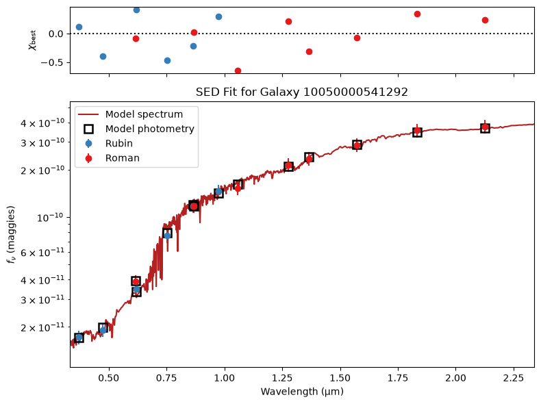
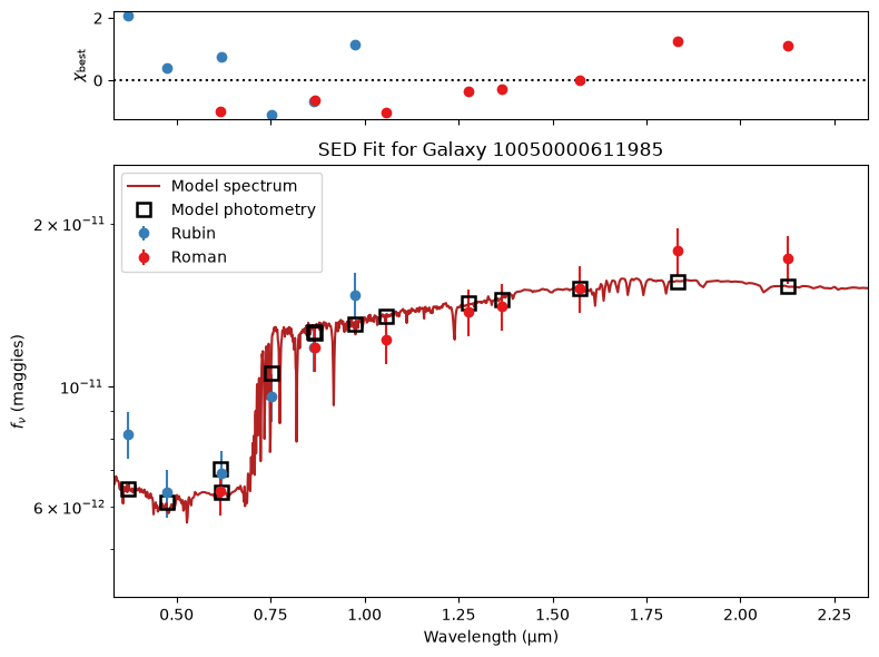
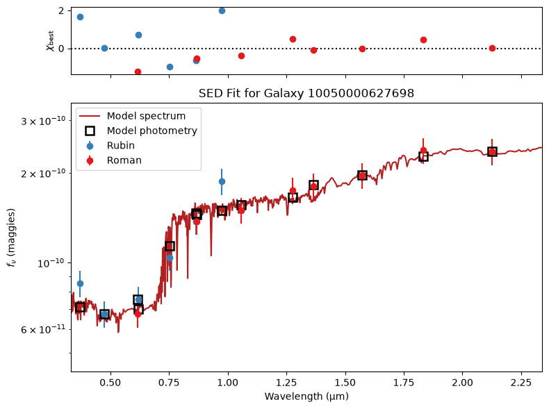
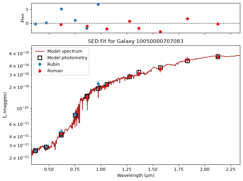
4.1 Plot the SEDs with their best fit from Prospector
Notebook Cell
def plot_SED_fit(outputs, obs_list, galaxy_id):
    """
    Plot SED fit for one galaxy in outputs/obs_list and print diagnostics.

    Parameters
    ----------
    outputs : list of dict
        Prospector output dicts (from fit_sample_parallel or load_outputs_and_obs).
    obs_list : list of dict
        Observation dicts, same order as outputs.
    galaxy_id : str or int
        Which galaxy to plot.

    Returns
    -------
    matplotlib.figure.Figure
        The SED fit figure.
    """
    # Locate this galaxy’s output and observation
    out = next((o for o in outputs if str(o.get("galaxy_id")) == str(galaxy_id)), None)
    obs = next((o for o in obs_list if str(o.get("galaxy_id")) == str(galaxy_id)), None)

    if out is None or obs is None:
        raise ValueError(f"Galaxy {galaxy_id} not found in outputs/obs_list")

    fig, (ax_resid, ax_sed) = plt.subplots(
        2, 1, gridspec_kw=dict(height_ratios=[1, 4]),
        sharex=True, figsize=(8, 6)
    )

    # Extract data
    pwave = np.array([f.wave_effective for f in obs["filters"]])
    bsed = out["bestfit"]
    obs_flux = np.array(obs["maggies"])
    obs_unc = np.array(obs["maggies_unc"])
    model_flux = np.array(bsed["photometry"])

    # Identify Rubin vs Roman filters by name
    filter_names = [f.name for f in obs["filters"]]
    rubin_mask = np.array(["lsst" in name.lower() for name in filter_names])
    roman_mask = np.array(["roman" in name.lower() for name in filter_names])

    # Convert model wavelengths from Å to µm for consistency with filter centers
    wavelengths_micron = bsed["restframe_wavelengths"] * (1 + obs["redshift"]) / 1e4
    pwave_micron = pwave / 1e4  # convert filter effective wavelengths too


    # --- lower panel: SED fit ---
    ax_sed.errorbar(
        pwave_micron[rubin_mask], obs_flux[rubin_mask], obs_unc[rubin_mask],
        fmt="o", color="#377eb8", label="Rubin"
    )
    ax_sed.errorbar(
        pwave_micron[roman_mask], obs_flux[roman_mask], obs_unc[roman_mask],
        fmt="o", color="#e41a1c", label="Roman"
    )

    # Overlay best-fit model spectrum
    ax_sed.plot(
        wavelengths_micron,
        bsed["spectrum"],
        color="firebrick",
        label="Model spectrum"
    )

    # model photometry: black boxes
    ax_sed.plot(
        pwave_micron, model_flux,
        "s", markersize=8, mec="k", mfc="none", mew=1.8, label="Model photometry"
    )

    # Y-axis scaling: tighten around data
    y_min = np.nanmin(obs_flux - 2 * obs_unc)
    y_max = np.nanmax(obs_flux + 2 * obs_unc)
    ax_sed.set_ylim(y_min * 0.8, y_max * 1.2)

    ax_sed.set_ylabel(r"$f_\nu$ (maggies)")
    ax_sed.set_xlabel(r"Wavelength (µm)")
    ax_sed.set_xlim(pwave_micron.min() * 0.9, pwave_micron.max() * 1.1)
    ax_sed.set_yscale("log")
    ax_sed.set_title(f"SED Fit for Galaxy {galaxy_id}", fontsize=12)
    ax_sed.legend(loc="best")

    # --- upper panel: residuals ---
    chi = (obs_flux - model_flux) / obs_unc
    # Separate Rubin and Roman photometric points for clarity
    ax_resid.errorbar(pwave_micron[rubin_mask], chi[rubin_mask], fmt="o", color="#377eb8")
    ax_resid.errorbar(pwave_micron[roman_mask], chi[roman_mask], fmt="o", color="#e41a1c")
    ax_resid.axhline(0, color="k", linestyle=":")
    ax_resid.set_ylabel(r"$\chi_{\rm best}$")

    fig.tight_layout()
    return
# Extract all galaxy IDs from the outputs list
galaxy_ids = [o["galaxy_id"] for o in outputs]
# Loop through each of the first 5 galaxy IDs and plot its SED fit
for gid in galaxy_ids[:5]:
plot_SED_fit(outputs, obs_list, gid)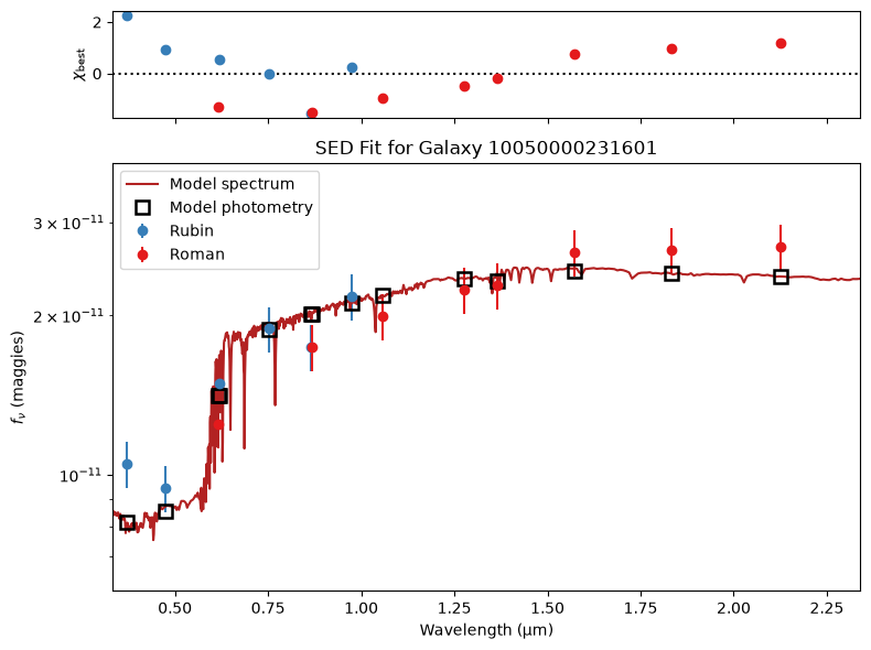
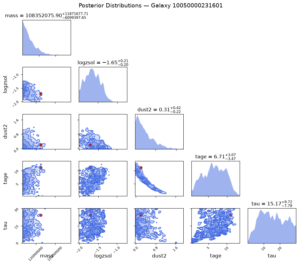
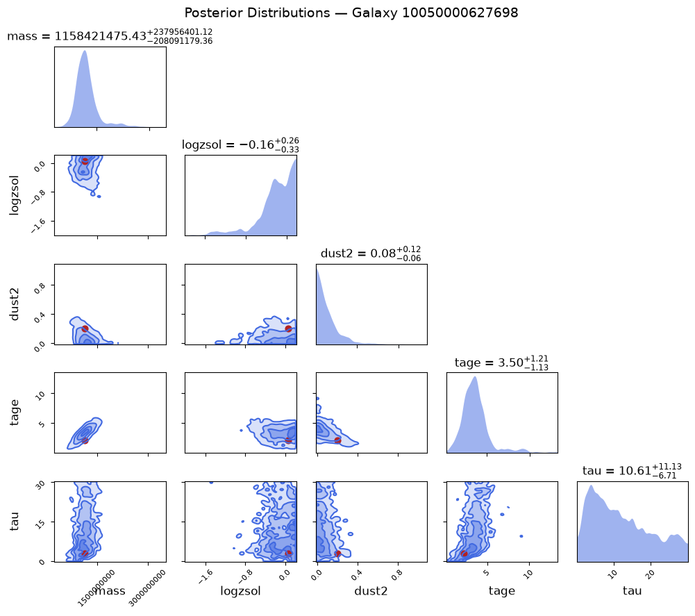
4.2 Plot corner plots of posteriors
Notebook Cell
def plot_corner(outputs, obs_list, galaxy_id):
    """
    Plot marginalized posterior corner diagram for one galaxy using Prospector's built-in corner plotting.

    Parameters
    ----------
    outputs : list of dict
        Processed Prospector output dicts (from fit_sample_parallel or load_outputs_hdf5).
    obs_list : list of dict
        Observation dicts (not used here, included for consistency).
    galaxy_id : str or int
        Galaxy ID to plot.

    Returns
    -------
    matplotlib.figure.Figure
        The corner plot figure showing marginalized posteriors.
    """
    color="royalblue"
    gid = str(galaxy_id)
    out = next((o for o in outputs if str(o.get("galaxy_id")) == gid), None)
    if out is None:
        raise ValueError(f"Galaxy {galaxy_id} not found in outputs")

    chain = out.get("chain")
    weights = out.get("weights")
    labels = out.get("theta_labels")

    if chain is None or weights is None or labels is None:
        raise ValueError(f"Output for galaxy {galaxy_id} missing chain/weights/labels")

    nsamples, ndim = chain.shape
    print(f"[Galaxy {galaxy_id}] Plotting corner with {nsamples} samples across {ndim} parameters")

    # Create subplots grid
    fig, axes = plt.subplots(ndim, ndim, figsize=(10, 9))

    # Plot using Prospector's built-in corner routine
    axes = corner.allcorner(
        chain.T,
        labels,
        axes,
        weights=weights,
        color=color,
        show_titles=True,
    )

    # Compute best sample manually if missing lnprobability
    if "lnprobability" in out and np.ndim(out["lnprobability"]) == 1:
        imax = np.argmax(out["lnprobability"])
        theta_best = chain[imax]
    elif "lnprobability" in out and np.ndim(out["lnprobability"]) == 2:
        # sometimes stored as sampler.logl per live point
        flat = out["lnprobability"].ravel()
        imax = np.argmax(flat)
        theta_best = chain[imax % len(chain)]
    else:
        # fallback to weighted best sample
        imax = np.argmax(weights)
        theta_best = chain[imax]

    # Overlay best-fit point
    from prospect.plotting import corner as pcorner
    pcorner.scatter(theta_best[:, None], axes, color="firebrick", marker="o", s=40)
    #pcorner.scatter(theta_best, axes,color="firebrick", marker="o", s=40)

    fig.suptitle(f"Posterior Distributions — Galaxy {galaxy_id}", fontsize=14)
    plt.tight_layout()
    plt.show()

    return
gid = galaxy_ids[0]
plot_corner(outputs, obs_list, gid)[Galaxy 10050000231601] Plotting corner with 1809 samples across 5 parameters
gid = galaxy_ids[3]
plot_corner(outputs, obs_list, gid)
[Galaxy 10050000627698] Plotting corner with 1884 samples across 5 parameters
5. Verification
As a sanity check, we compare the stellar masses derived by Prospector to the “true” simulated stellar masses stored in the OpenUniverse catalog. Agreement along the 1:1 line indicates successful recovery of physical parameters.
Notebook Cell
def plot_stellar_mass_verification(df, outputs):
    """
    Verify measured stellar mass against input stellar mass for multiple galaxies.

    Parameters
    ----------
    df : pandas.DataFrame
        DataFrame containing the true/input stellar masses. Must include
        a column "um_source_galaxy_obs_sm".
    outputs : list of dict
        List of processed Prospector results dicts (from process_output).

    Returns
    -------
    matplotlib.figure.Figure
        The verification plot figure.
    """

    # Extract input (true) stellar masses from the catalog
    input_mass = df["um_source_galaxy_obs_sm"].values
    print("Input mass", input_mass)

    # Initialize lists to store median and uncertainty for each galaxy
    measured_mass, err_low, err_high = [], [], []

    # Loop through all Prospector fit results
    for out in outputs:

        # Extract the MCMC chain and parameter names
        chain = out["chain"]
        param_names = out["theta_labels"]

        # Identify the 'mass' parameter index (log10 of stellar mass)
        idx = param_names.index("mass")  #is in logmass

        # Convert log(mass) samples to linear scale (M☉)
        samples = np.log10(chain[:, idx])  # convert to log
        mass_samples = 10 ** samples  # in M☉

        # Compute median and 16th/84th percentiles as uncertainty bounds
        median = np.median(mass_samples)
        low, high = np.percentile(mass_samples, [16, 84])

        # Store median and asymmetric error bars
        measured_mass.append(median)
        err_low.append(median - low)
        err_high.append(high - median)

    # --- plotting ---
    fig, ax = plt.subplots(figsize=(6, 6))
    ax.errorbar(input_mass, measured_mass,
                yerr=[err_low, err_high],
                fmt="o", color="royalblue", ecolor="lightgray", alpha=0.7)

    #make the 1:1 correlation line
    lims = [min(input_mass.min(), min(measured_mass)),
            max(input_mass.max(), max(measured_mass))]
    ax.plot(lims, lims, "k--")
    ax.set_xscale("log")
    ax.set_yscale("log")

    ax.set_xlabel("Input stellar mass")
    ax.set_ylabel("Measured stellar mass")
    ax.set_title("Stellar Mass Verification")

    return
plot_stellar_mass_verification(df_small, outputs)Input mass [1.94016064e+08 9.80352560e+07 2.43979584e+08 2.17925312e+08
1.07500816e+08 1.29884296e+08 1.43338496e+09 3.64248218e+09
3.90629811e+09 7.93237632e+08 1.13509094e+09 4.91075400e+07
3.30186720e+08 2.97556429e+09 1.25218163e+09 2.22853530e+09
8.18764400e+07 6.56323277e+09 2.43161984e+09 7.62999347e+09]
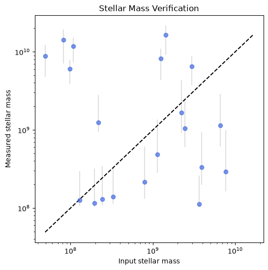
The example shown here does not yield particularly accurate stellar‐mass estimates — this is understandable given the simplifying assumptions used in the tutorial. As noted in the Assumptions section above, these quick Prospector runs are intended to demonstrate how to use and visualize OpenUniverse data rather than to optimize astrophysical fits. Users are encouraged to experiment with model parameters, priors, and error settings to obtain more realistic results.
6. Host galaxy properties as a function of SN type
Finally, we examine whether host galaxy properties differ between Type Ia and Core-Collapse supernovae. We compare the distribution of Prospector-derived stellar masses for the two SN classes.
Notebook Cell
def plot_1a_vs_cc_mass(df_sn, outputs):
    """
    Plot histograms of Prospector-fitted host stellar masses for
    Type Ia vs Core-Collapse (CC) supernova hosts.

    Parameters
    ----------
    df_sn : pandas.DataFrame
        Must contain columns 'model_name' and either 'id' or 'galaxy_id'.
        'model_name' is used to classify SN type.
    outputs : list of dict
        Processed Prospector outputs (from process_output), one per galaxy.
        Must contain keys: 'galaxy_id', 'chain', and 'theta_labels'.

    Notes
    -----
    - Stellar mass in Prospector is stored as log10(M/M☉).
    - 'SALT3.NIR_WAVEEXT' is treated as Type Ia.
    - All other SN models are grouped as Core-Collapse.
    """

    # --- extract stellar masses from Prospector outputs ---
    prospector_masses = []
    for out in outputs:

        # Extract the MCMC chain and parameter names
        chain = out["chain"]
        param_names = out["theta_labels"]
        gid = str(out["galaxy_id"])  # ensure string for consistency

        if "mass" not in param_names:
            print(f"[warning] Galaxy {gid} has no 'mass' parameter; skipping.")
            continue

        # Identify the 'mass' parameter index (log10 of stellar mass)
        idx = param_names.index("mass")
        logmass_samples = chain[:, idx]
        logmass_median = np.median(logmass_samples)
        prospector_masses.append(dict(galaxy_id=gid, log_mass=logmass_median))

    df_mass = pd.DataFrame(prospector_masses)

    # --- ensure consistent dtype for merge keys ---
    df_sn = df_sn.copy()
    df_sn["galaxy_id"] = df_sn["galaxy_id"].astype(str)
    df_mass["galaxy_id"] = df_mass["galaxy_id"].astype(str)

    # --- merge ---
    merged = df_sn.merge(df_mass, left_on="galaxy_id", right_on="galaxy_id", how="inner")

    if merged.empty:
        raise ValueError("[error] No matches found between df_sn and Prospector outputs. Check ID formats.")

    # --- classify SN types ---
    merged["SN_type"] = merged["model_name"].apply(
        lambda m: "Type Ia" if m == "SALT3.NIR_WAVEEXT" else "Core-Collapse"
    )

    # --- plot ---
    plt.figure(figsize=(8, 5))
    sn_types = merged["SN_type"].unique()

    if len(sn_types) > 1:
        # Two or more SN types → overlay histograms
        sns.histplot(
            data=merged,
            x="log_mass",
            hue="SN_type",
            multiple="layer",
            stat="density",
            common_norm=False,
            palette={"Type Ia": "tab:blue", "Core-Collapse": "tab:orange"},
            bins=20
        )
        plt.title("Prospector-Derived Host Stellar Mass:\nType Ia vs Core-Collapse SNe")
        # ensure legend always appears
        handles, labels = plt.gca().get_legend_handles_labels()
        if not labels:
            plt.legend(["Type Ia", "Core-Collapse"], title="SN Type", loc="best")
        else:
            plt.legend(title="SN Type", loc="best")
    else:
        # Only one SN type → single histogram, fixed color
        single_type = sn_types[0]
        color = "tab:blue" if single_type == "Type Ia" else "tab:orange"
        sns.histplot(
            data=merged,
            x="log_mass",
            color=color,
            element="step",
            stat="density",
            bins=20
        )
        plt.title(f"Prospector-Derived Host Stellar Mass ({single_type} Only)")

    plt.xlabel(r"Host Stellar Mass $\log_{10}(M_*/M_\odot)$ (Prospector fit)")
    plt.ylabel("Normalized Density")
    plt.tight_layout()
    plt.show()
plot_1a_vs_cc_mass(df_sn, outputs)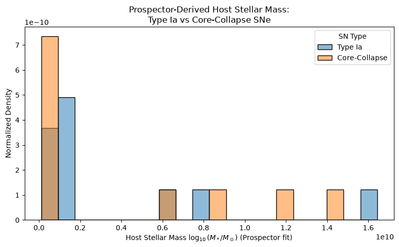
Distribution of Prospector-derived host galaxy stellar masses for Type Ia and Core-Collapse supernovae. The two distributions do not show a clear separation, which likely reflects the limited accuracy of the stellar-mass fits in this quick demonstration. As discussed in the stellar-mass verification figure (Section 5), the simplified assumptions used in the tutorial—such as fixed flux uncertainties and basic model priors—introduce significant scatter that can obscure any underlying physical differences between the SN host populations. Larger sample sizes or more attention to fit assumptions may clarify this plot.
Acknowledgements
About this notebook
Authors: Jessica Krick, Jaladh Singhal, Brigitta Sipőcz
Updated: 2026-02-12
Contact: IRSA Helpdesk with questions or problems.
Runtime: As of the date above, this notebook takes about 70s to run to completion on a machine with 8GB RAM and 2 CPU without running any of the SED fitting. Running this tutorial including fitting on 20 galaxies takes about 40 minutes to run to completion on a machine with 64GB RAM and 16 CPU.
AI Acknowledgement: This tutorial was developed with the assistance of OpenAI’s ChatGPT (GPT-5)
References
Johnson, B. D., Leja, J., Conroy, C., & Speagle, J. S. (2021). Stellar Population Inference with Prospector. The Astrophysical Journal Supplement Series, 254(2), 22.
Leja, J., Johnson, B. D., Conroy, C., van Dokkum, P. G., & Byler, N. (2017). An Older, More Quiescent Universe from Panchromatic SED Fitting of the 3D-HST Survey. The Astrophysical Journal, 837 (2), 170.
Conroy, C., Gunn, J. E., & White, M. (2009). The Propagation of Uncertainties in Stellar Population Synthesis Modeling. The Astrophysical Journal, 699(1), 486–506.
Conroy, C., & Gunn, J. E. (2010). The Propagation of Uncertainties in Stellar Population Synthesis Modeling. II. The Challenge of Comparing Galaxy Evolution Models to Observations. The Astrophysical Journal, 712(2), 833–857.
Johnson, B. D. (2024). python-fsps: Python bindings to the Flexible Stellar Population Synthesis (FSPS) code (Version 0.4.7) Computersoftware. Zenodo. Ben Johnson et al. (2024)
Speagle, J. S. (2020). DYNESTY: a dynamic nested sampling package for estimating Bayesian posteriors and evidences. Monthly Notices of the Royal Astronomical Society, 493(3), 3132–3158.
Speagle, J. S. (2025). dynesty: Dynamic Nested Sampling in Python (Version 2.1.0) Computersoftware. Zenodo. Sergey Koposov et al. (2025)
Foreman-Mackey, D., Hogg, D. W., Lang, D., & Goodman, J. (2013). emcee: The MCMC Hammer. Publications of the Astronomical Society of the Pacific, 125(925), 306–312.
The Roman Supernova Cosmology Project Infrastructure Team (2025). OpenUniverse2024: A shared, simulated view of the sky for the next generation of cosmological surveys. Monthly Notices of the Royal Astronomical Society, 1729T. Open Universe Team (2025)
print("total time", time.time() - starttime)total time 27.324543237686157
- Ben Johnson, Dan Foreman-Mackey, Jonathan Sick, Joel Leja, Mike Walmsley, Erik Tollerud, Henry Leung, Spencer Scott, & Minjung Park. (2024). dfm/python-fsps: v0.4.7. Zenodo. 10.5281/ZENODO.12447779
- Sergey Koposov, Josh Speagle, Kyle Barbary, Gregory Ashton, Ed Bennett, Johannes Buchner, Carl Scheffler, Colm Talbot, Ben Cook, James Guillochon, Patricio Cubillos, Andrés Asensio Ramos, Matthieu Dartiailh, Ilya, Erik Tollerud, Dustin Lang, Ben Johnson, jtmendel, Edward Higson, … joezuntz. (2025). joshspeagle/dynesty: v3.0.0. Zenodo. 10.5281/ZENODO.17268284
- Open Universe Team. (2025). OpenUniverse 2024 Simulated Roman and Rubin Images: Full Area. IPAC. 10.26131/IRSA596