Learning Goals
By the end of this tutorial, you will be able to :
Query the OpenUniverse2024 images for a source of interest
Perform aperture photometry on images
Generate a light curve
Display full images and cutouts
Introduction
The OpenUniverse2024 simulation suite delivers ~70 deg² of matched optical/infrared imagery designed for both the LSST Wide‑Fast‑Deep (WFD) and the Nancy Grace Roman Space Telescope high-latitude survey, enabling joint survey planning and multi-wavelength systematics studies. It incorporates the updated “Diffsky” extragalactic model, extended transient modeling across optical/IR wavelengths, and realistic telescope/instrument effects, producing roughly 400 TB of publicly available synthetic imaging and catalogs. The goal of this project is to enable cross-collaboration and maximize science return from next-generation cosmological surveys by providing a consistent simulated sky observed by multiple observatories.
Tidal Disruption Events (TDEs) occur when a star passes close enough to a supermassive black hole to be torn apart by tidal forces, producing a luminous flare that can outshine the host galaxy for weeks to months. Identifying and characterizing TDE host galaxies is key to understanding the demographics of supermassive black holes and the galactic environments that produce these rare events. This notebook demonstrates how to locate a simulated TDE from the OpenUniverse2024 transient input catalog, identify its host galaxy, and extract optical and infrared photometry from Roman images to construct a multi-epoch light curve. The OpenUniverse2024 dataset also provides matched Rubin optical coverage over the same sky. With a few simple changes in Sections 3 and 4, this workflow can be extended to other Roman and Rubin bands to build a true multi-wavelength light curve.
Instructions
This notebook is designed to be run sequentially from top to bottom. All code is self-contained and relies on publicly accessible data.
Input
A TDE from the OpenUniverse2024 transient input catalog
Output
Light curve(s) of host galaxy(s)
Cutout gallery of host galaxy(s)
Imports
# Uncomment the next line to install dependencies if needed.
# !pip install numpy astropy s3fs photutils matplotlib scipy pandas fsspec pyarrow hpgeom astroquery
from astropy.io import fits
import numpy as np
import s3fs
from matplotlib import pyplot as plt
import pandas as pd
from photutils.aperture import SkyCircularAperture, SkyCircularAnnulus, aperture_photometry, ApertureStats
from scipy.ndimage import rotate
from astropy import units as u
from astropy.coordinates import SkyCoord
from astropy.nddata import Cutout2D
from astropy.wcs import WCS
import pyarrow.dataset as ds
import pyarrow.fs
import pyarrow.parquet as pq
import hpgeom
import json
from astroquery.ipac.irsa import Irsa
import itertools/home/runner/work/irsa-tutorials/irsa-tutorials/.tox/py312-buildhtml/lib/python3.12/site-packages/tqdm/auto.py:21: TqdmWarning: IProgress not found. Please update jupyter and ipywidgets. See https://ipywidgets.readthedocs.io/en/stable/user_install.html
from .autonotebook import tqdm as notebook_tqdm
1. Explore the OpenUniverse2024 data directories
This section of the tutorial demonstrates how to explore the OpenUniverse2024 data directories directly on S3 and inspect simulated Roman and Rubin images without downloading large datasets locally. It establishes a connection to the public NASA IRSA simulations bucket using s3fs, defines key directory paths for the full Roman and Rubin simulations, and illustrates how to browse image files for a selected band and pointing. The accompanying functions — summarize_fits_files() and show_gallery() — provide tools for quickly summarizing FITS file metadata (e.g., number of extensions, pointing information, pixel scale) and for visualizing a small gallery of example images from the chosen directory.
In the prefix you will see that we choose “simple_model” simulations and not “truth” simulations because the simple_model images are the ones with noise and real effects, while “Truth” are noise free, perfect images.
The prefix also selects the full simulation, which covers the entire survey footprint, for both Roman and Rubin. The OpenUniverse2024 paper describes how the simulation was produced.
# Setup

# Create a connection to the public NASA IRSA S3 storage bucket using the `s3fs` library.
# By setting `anon=True`, the connection is opened in **anonymous read-only mode**,
# allowing us to list and access public files (such as the OpenUniverse2024 Roman and
# Rubin simulation data) directly from S3 without requiring AWS credentials.

#initialize a general interface to Amazon cloud
s3 = s3fs.S3FileSystem(anon=True)

#general location information
BUCKET_NAME = "nasa-irsa-simulations"
OU_PREFIX = "openuniverse2024"
ROMAN_TDS_PREFIX = "roman/full/RomanTDS/images/simple_model"  #
CATALOG_NAME = "roman_rubin_cats_v1.1.2_faint"

#spcific location information
BAND= "J129"
POINTING = "10190"

#the full path to the data we are interested in exploring
image_directory = f"{BUCKET_NAME}/{OU_PREFIX}/{ROMAN_TDS_PREFIX}/{BAND}/{POINTING}"

#list the contents
s3.ls(image_directory)
['nasa-irsa-simulations/openuniverse2024/roman/full/RomanTDS/images/simple_model/J129/10190/Roman_TDS_simple_model_J129_10190_1.fits.gz',
'nasa-irsa-simulations/openuniverse2024/roman/full/RomanTDS/images/simple_model/J129/10190/Roman_TDS_simple_model_J129_10190_10.fits.gz',
'nasa-irsa-simulations/openuniverse2024/roman/full/RomanTDS/images/simple_model/J129/10190/Roman_TDS_simple_model_J129_10190_11.fits.gz',
'nasa-irsa-simulations/openuniverse2024/roman/full/RomanTDS/images/simple_model/J129/10190/Roman_TDS_simple_model_J129_10190_12.fits.gz',
'nasa-irsa-simulations/openuniverse2024/roman/full/RomanTDS/images/simple_model/J129/10190/Roman_TDS_simple_model_J129_10190_13.fits.gz',
'nasa-irsa-simulations/openuniverse2024/roman/full/RomanTDS/images/simple_model/J129/10190/Roman_TDS_simple_model_J129_10190_14.fits.gz',
'nasa-irsa-simulations/openuniverse2024/roman/full/RomanTDS/images/simple_model/J129/10190/Roman_TDS_simple_model_J129_10190_15.fits.gz',
'nasa-irsa-simulations/openuniverse2024/roman/full/RomanTDS/images/simple_model/J129/10190/Roman_TDS_simple_model_J129_10190_16.fits.gz',
'nasa-irsa-simulations/openuniverse2024/roman/full/RomanTDS/images/simple_model/J129/10190/Roman_TDS_simple_model_J129_10190_17.fits.gz',
'nasa-irsa-simulations/openuniverse2024/roman/full/RomanTDS/images/simple_model/J129/10190/Roman_TDS_simple_model_J129_10190_18.fits.gz',
'nasa-irsa-simulations/openuniverse2024/roman/full/RomanTDS/images/simple_model/J129/10190/Roman_TDS_simple_model_J129_10190_2.fits.gz',
'nasa-irsa-simulations/openuniverse2024/roman/full/RomanTDS/images/simple_model/J129/10190/Roman_TDS_simple_model_J129_10190_3.fits.gz',
'nasa-irsa-simulations/openuniverse2024/roman/full/RomanTDS/images/simple_model/J129/10190/Roman_TDS_simple_model_J129_10190_4.fits.gz',
'nasa-irsa-simulations/openuniverse2024/roman/full/RomanTDS/images/simple_model/J129/10190/Roman_TDS_simple_model_J129_10190_5.fits.gz',
'nasa-irsa-simulations/openuniverse2024/roman/full/RomanTDS/images/simple_model/J129/10190/Roman_TDS_simple_model_J129_10190_6.fits.gz',
'nasa-irsa-simulations/openuniverse2024/roman/full/RomanTDS/images/simple_model/J129/10190/Roman_TDS_simple_model_J129_10190_7.fits.gz',
'nasa-irsa-simulations/openuniverse2024/roman/full/RomanTDS/images/simple_model/J129/10190/Roman_TDS_simple_model_J129_10190_8.fits.gz',
'nasa-irsa-simulations/openuniverse2024/roman/full/RomanTDS/images/simple_model/J129/10190/Roman_TDS_simple_model_J129_10190_9.fits.gz']# open and explore extensions
# how many files are in the bucket?
files = [f"s3://{f}" for f in s3.ls(image_directory)]
print(f"Found {len(files)} files")
#pick one fits file to explore
fname = files[0]
#describe the available extensions in this fits file
with fits.open(fname, use_fsspec=True, fsspec_kwargs={"anon": True}, memmap=False) as hdul:
print(f"File: {fname}")
print(f"Number of extensions: {len(hdul)}\n")
hdul.info()Found 18 files
File: s3://nasa-irsa-simulations/openuniverse2024/roman/full/RomanTDS/images/simple_model/J129/10190/Roman_TDS_simple_model_J129_10190_1.fits.gz
Number of extensions: 4

Filename: <class 's3fs.core.S3File'>
No.    Name      Ver    Type      Cards   Dimensions   Format
  0  PRIMARY       1 PrimaryHDU      63   ()
  1  SCI           1 ImageHDU        68   (4088, 4088)   float64
  2  ERR           1 ImageHDU        68   (4088, 4088)   float32
  3  DQ            1 ImageHDU        70   (4088, 4088)   int32 (rescales to uint32)
This output lists the structure and contents of one example Roman TDS FITS image from the OpenUniverse2024 dataset. It shows that 18 image files were found in the selected directory, and the examined file contains four extensions: a primary header (no data) followed by three 4088×4088 pixel image planes labeled SCI, ERR, and DQ, which store the science image, per-pixel uncertainty, and data quality mask, respectively. For each extension, the output reports its type, data dimensions, and the first few header keywords to give you a sense of what is in the file.
Let’s take a look at a few images to see what we are dealing with.
Notebook Cell
def show_gallery(files, max_images=9):
    """
    Display a gallery of FITS images.

    Parameters
    ----------
    files : list of str
        List of S3 URIs to FITS files.
    max_images : int, optional
        Maximum number of images to display (default: 9).
    """
    # Limit the number of images to display
    n_images = min(len(files), max_images)

    # Choose number of columns: up to 3, or equal to n_images if fewer than 4
    ncols = n_images if n_images < 4 else 3

    # Compute number of rows based on total images and columns
    nrows = (n_images + ncols - 1) // ncols

    # Create the subplot grid
    fig, axes = plt.subplots(nrows, ncols, figsize=(4 * ncols, 4 * nrows))
    axes = np.atleast_1d(axes).ravel()  # flatten in case of 1D output

    # Loop through each file and display the image
    for i, f in enumerate(files[:n_images]):
        # Open FITS file directly from S3 (anonymous read)
        with fits.open(f, fsspec_kwargs={"anon": True}, memmap=False) as hdul:
            data = hdul[1].data  # Extract image data
            # Compute robust display scaling (5th–99th percentile)
            vmin, vmax = np.nanpercentile(data, [5, 99])
            # Show image in grayscale with good contrast
            axes[i].imshow(data, origin="lower", cmap="gray", vmin=vmin, vmax=vmax)
            del data
            # Title: just the base filename
            axes[i].set_title(f.split("/")[-1], fontsize=8)
            # Remove tick marks and labels
            axes[i].axis("off")

    # Hide any unused subplot axes
    for j in range(i + 1, len(axes)):
        axes[j].axis("off")

    # Adjust layout for neat display
    plt.tight_layout()
    plt.show()
# Number of example images to display. Increase to see more of the available images.
n_gallery_images = 4
show_gallery(files, max_images=n_gallery_images)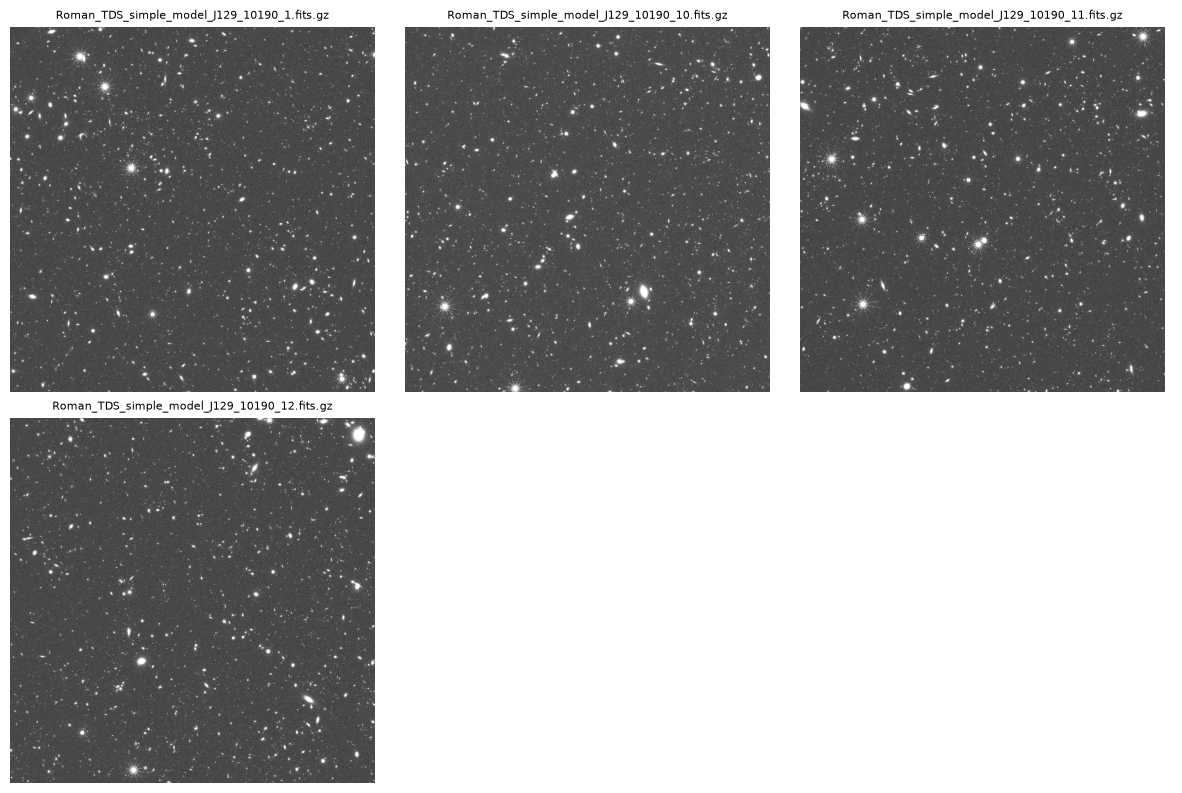
2. Find a TDE target from the transient catalog
We use the OpenUniverse2024 transient input catalog — the same SNANA parquet files described in the SED Fitting tutorial — to find a TDE. The catalog stores one parquet file per HEALPix region, and TDEs are rare, so not every region will contain one. The catalog is split into three types of parquet files, each indexed by HEALPix region:
snana_{region}.parquet — the transient source catalog, with one row per simulated event (supernovae, TDEs, etc.), including fields such as the event type (model_name) and the ID of the host galaxy (host_id)
galaxy_{region}.parquet — the host galaxy catalog, with sky positions and physical properties for each galaxy
galaxy_flux_{region}.parquet — multi-band photometry for each galaxy (used in the SED Fitting tutorial but not needed here)
TDEs are rare, so not every region will contain one. We use the known center of the Roman Time-Domain Survey to target the right region directly. We then cross-match the TDE’s host_id into the galaxy file to retrieve the host’s sky coordinates for the image search that follows.
First, we connect to S3 and list all available SNANA parquet files in the catalog.
fs = pyarrow.fs.S3FileSystem(region='us-east-1', anonymous=True)
catalog_prefix = f"{BUCKET_NAME}/{OU_PREFIX}/roman/full/{CATALOG_NAME}"

# List all SNANA parquet files in the catalog directory, sorted for consistent ordering.
file_info = fs.get_file_info(pyarrow.fs.FileSelector(catalog_prefix, recursive=False))
snana_files = sorted([
    f.path for f in file_info
    if f.base_name.startswith("snana_") and f.base_name.endswith(".parquet")
])

print(f"Found {len(snana_files)} snana parquet files")
Found 33 snana parquet files
Since our goal is to make a light curve for a TDE, we need to pick a SNANA parquet file that is covered by the Roman Time-Domain Survey (TDS).
# Time Domain Survey (TDS) is centered at LSST ELAIS-S1 DDF:
ra = 9.45
dec = -44.02

# In snana_{region}.parquet, region is HEALPix pixel ID at order 5 (nside=32) with RING ordering
nside = 32
nest = False

# Convert TDS center coordinates to region ID used in the naming of SNANA parquet files
region = hpgeom.angle_to_pixel(nside, ra, dec, lonlat=True, nest=False)
snana_path = [f for f in snana_files if f"snana_{region}.parquet" in f][0]
snana_path'nasa-irsa-simulations/openuniverse2024/roman/full/roman_rubin_cats_v1.1.2_faint/snana_10307.parquet'Next, we scan this file and find a row with model_name == "NON1ASED.TDE-BBFIT" that represents a TDE.
# Read the parquet file into a pandas dataframe.
df = pq.read_table(snana_path, filesystem=fs).to_pandas()
# Look for TDE models.
mask = df["model_name"] == "NON1ASED.TDE-BBFIT"
if mask.any():
   # Choose the first TDE
    tde_info = df[mask].iloc[0].squeeze()
    print(f"Found a TDE in region {region} with the following info:")
    print(tde_info)
else:
    raise RuntimeError(f"No TDE found in region {region}.")
Found a TDE in region 10307 with the following info:
id 110000037
ra 11.026759
dec -43.406039
host_id 10307000012568
gentype 42
model_name NON1ASED.TDE-BBFIT
start_mjd 62228.0
end_mjd 62432.0
z_CMB 0.2397
mw_EBV 0.0
mw_extinction_applied False
AV -9.0
RV -9.0
v_pec 0.0
host_ra 11.02676
host_dec -43.406045
host_mag_g 22.708
host_mag_i 22.01
host_mag_F 21.459
host_sn_sep 0.021294
peak_mjd 62240.375
peak_mag_g 22.402536
peak_mag_i 22.951426
peak_mag_F 24.470018
lens_dmu 0.0
lens_dmu_applied False
model_param_names [template_index]
model_param_values [1.0]
MW_av 0.02339
MW_rv 3.1
Name: 62959, dtype: object
Once we have the TDE, we load the corresponding galaxy info parquet file for that region. Then we identify its host galaxy(s) by matching the host ID in the TDE info with the galaxy IDs in the galaxy info.
galaxy_info_file = f"{catalog_prefix}/galaxy_{region}.parquet"
host_galaxy = pq.read_table(galaxy_info_file, filesystem=fs,
                              # filter while reading pq for time efficiency
                              filters=[("galaxy_id", "==", tde_info["host_id"])]
                              ).to_pandas()
host_galaxy3. Image Access
Now we have the host galaxy’s position and ID in host_galaxy, ready for image queries. With those coordinates in hand, we then query the Roman image files that overlap this region, retrieving only the files needed for subsequent photometry and light-curve analysis.
# Point the astroquery IRSA client to the correct locations.
Irsa.sia_url = "https://irsa.ipac.caltech.edu/simulated/SIA"
Irsa.tap_url = "https://irsa.ipac.caltech.edu/simulated/TAP"

Irsa.list_collections(servicetype='SIA')OU_ROMAN_SIA_COLLECTION = 'simulated_roman_openuniverse2024'
OU_RUBIN_SIA_COLLECTION = 'simulated_rubin_openuniverse2024'Notebook Cell
def get_s3_fpath(cloud_access):
    """Extract the S3 URI from the cloud_access JSON string in an SIA result."""
    cloud_info = json.loads(cloud_access) # converts str to dict
    bucket_name = cloud_info['aws']['bucket_name']
    key = cloud_info['aws']['key']

    return f's3://{bucket_name}/{key}'
First, we find the filenames of the images in the Roman TDS survey which include the TDE host galaxy.
Notebook Cell
def Roman_TDS_image_search(host_galaxy, radius, bandname):
    """
    Get OpenUniverse2024 Roman TDS images for the TDE host galaxy.

    Parameters
    ----------
    host_galaxy : pandas.DataFrame
        Must include 'galaxy_id', 'ra', and 'dec' columns.
    radius : astropy.units.Quantity
        Search radius.
    bandname : string
        Roman bandname for which to search images (e.g. 'J129', 'H158').

    Returns
    -------
    astropy.table.Table
        SIA result table filtered to TDE images in the specified band,
        with an added 's3_uri' column for the image file paths.
    """
    row = host_galaxy.iloc[0]
    galaxy_id = int(row["galaxy_id"])
    ra_center, dec_center = row["ra"], row["dec"]
    print(f"Accessing images in band={bandname} for galaxy_id={galaxy_id} at RA={ra_center:.3f}, Dec={dec_center:.3f} ...", end="")

    coords = SkyCoord(ra_center, dec_center, unit='deg')
    sia_results = Irsa.query_sia(pos=(coords, radius.to(u.deg)), collection=OU_ROMAN_SIA_COLLECTION)
    filtered_results = sia_results[['TDS_simple_model' in r['obs_id'] and bandname in r['energy_bandpassname']
                                    for r in sia_results]]
    filtered_results['s3_uri'] = [get_s3_fpath(r['cloud_access']) for r in filtered_results]

    print(f"done. Found {len(filtered_results)} images.")
    return filtered_results
bands = ["J129", "H158"]
image_search_radius = 1 * u.arcsec # point-like since we just need images containing the host galaxy
all_band_images = {}
for bandname in bands:
all_band_images[bandname] = Roman_TDS_image_search(host_galaxy, image_search_radius, bandname)Accessing images in band=J129 for galaxy_id=10307000012568 at RA=11.027, Dec=-43.406 ...done. Found 173 images.
Accessing images in band=H158 for galaxy_id=10307000012568 at RA=11.027, Dec=-43.406 ...done. Found 166 images.
Since there are > 100 TDS images per band, we will:
restrict to images taken during the TDE event window (
start_mjdtoend_mjdfrom the transient catalog) so the light curve focuses on the TDE itself rather than the full survey duration.filter out images where the host galaxy is close to the edge so that photometry is more reliable and partial cutouts can be avoided.
select only an evenly time-sampled subset of images so that photometry is quicker to run.
Notebook Cell
def select_images_by_mjd_quantiles(images, n_select=9):
    """
    Select up to `n_select` images using rank-quantiles on time axis.

    Parameters
    ----------
    images : astropy Table
        Table of images (SIA results).
    n_select : int, optional
        Maximum number of images to select. Default is 9.

    Returns
    -------
    astropy Table
        Subset of input `images` corresponding to the selected quantiles.
    """
    sorted_images = images.copy()  # avoid modifying the original table
    sorted_images.sort('t_min') # sort by time axis, t_min = t_max for TDS images, so we can use either
    num_quantiles = min(n_select, len(sorted_images))
    quantile_indices = np.rint(  # round off to nearest integer
        np.linspace(0, len(sorted_images) - 1, num_quantiles)
    ).astype(int)
    return sorted_images[quantile_indices]
galaxy_id = int(host_galaxy.iloc[0]["galaxy_id"])
host_coord = SkyCoord(host_galaxy.iloc[0]["ra"], host_galaxy.iloc[0]["dec"], unit='deg')
for bandname in bands:
image_tbl = all_band_images[bandname]
# 1. restrict to images within the TDE event window
tde_start, tde_end = tde_info["start_mjd"], tde_info["end_mjd"]
in_window = [tde_start <= r['t_min'] <= tde_end for r in image_tbl]
selected_images = image_tbl[in_window]
# 2. filter out images where the host galaxy falls near the edge
# 's_fov' is the estimated diameter of the image, so 0.45 * s_fov is 90% of its radius.
# Keep images where the host galaxy sits closer than that to the center ('s_ra', 's_dec').
image_centers = SkyCoord(selected_images['s_ra'], selected_images['s_dec'], unit='deg')
dist_to_center = host_coord.separation(image_centers).deg
not_on_edge = dist_to_center < (0.45 * selected_images['s_fov'])
selected_images = selected_images[not_on_edge]
# 3. select an evenly time-sampled subset
selected_images = select_images_by_mjd_quantiles(selected_images)
print(f"Band {bandname}, Galaxy {galaxy_id}: Downsampled {len(image_tbl)} images to {len(selected_images)} images.")
# store per-band image filenames as a band-specific column
host_galaxy[f"image_filenames_{bandname}"] = [selected_images['s3_uri'].tolist()]Band J129, Galaxy 10307000012568: Downsampled 173 images to 9 images.
Band H158, Galaxy 10307000012568: Downsampled 166 images to 9 images.
# check if we have a nested column of image filenames for the host galaxy
host_galaxy4. Make a Light Curve
This section demonstrates how to extract and visualize a light curve for a Tidal Disruption Event using simulated Roman images in two bands (J129 and H158).
The first function, run_aperture_photometry(), performs simple circular aperture photometry on a set of FITS images from S3 using the astropy photutils package.
The two plotting functions then compile these measurements into time-ordered plots showing how the observed flux evolves across multiple visits, providing a first look at temporal variability that could signal transient activity or host-galaxy changes.
Notebook Cell
def run_aperture_photometry(host_galaxy, bandname, image_column="image_filenames", aperture_radius=1.0):
    """
    Perform circular aperture photometry on a list of FITS images.

    Parameters
    ----------
    host_galaxy : pandas.DataFrame
        Must contain columns 'ra', 'dec', and a nested column with FITS image paths
        (each a list of FITS image paths).
    bandname : string
        Bandname for which to do photometry.
    image_column : string, optional
        Name of the dataframe column containing lists of FITS image paths.
        Default is "image_filenames".
    aperture_radius : float, optional
        Aperture radius in arcsec. Default is 1.0 arcseconds which is ~9 pixels for Roman .

    Returns
    -------
    None
        Results are added directly to `host_galaxy` as new columns:
        f'mjd_obs_{{bandname}}', f'flux_{{bandname}}', f'flux_err_{{bandname}}',
        and 'aperture_radius_pix'.
    """

    row = host_galaxy.iloc[0]
    filenames = row[image_column]
    print(f"Performing photometry in {bandname} for {len(filenames)} sampled images "
          f"for host galaxy at RA={row['ra']:.3f}, Dec={row['dec']:.3f} ...", end="")

    mjd_list, flux_list, flux_err_list, aperture_radius_pix_list = [], [], [], []

    for fname in filenames:

        #opening a gzipped fits file, don't recommend changing the next line.
        with fits.open(fname, fsspec_kwargs={"anon": True}, memmap=False) as hdul:
            data = hdul[1].data
            header = hdul[1].header

            # Build a WCS object so photutils can convert between sky and pixel coordinates.
            wcs = WCS(header)

            # Simple circular aperture centered on the host galaxy position
            sky_position = SkyCoord(row["ra"], row["dec"], unit="deg", frame="icrs")
            aperture = SkyCircularAperture(sky_position, r=aperture_radius * u.arcsec)
            pixel_aperture = aperture.to_pixel(wcs)

            # Perform aperture photometry
            phot_table = aperture_photometry(data, aperture, wcs=wcs)

            # Check output (optional)
            #print(phot_table)

            # Background estimate from a local annulus around the source
            annulus = SkyCircularAnnulus(sky_position, r_in=3 * aperture_radius * u.arcsec,
                                                       r_out=6 * aperture_radius * u.arcsec)
            annulus_stats = ApertureStats(data, annulus, wcs=wcs)
            background = annulus_stats.median

            # Subtract background from aperture sum
            aperture_area = pixel_aperture.area
            flux = phot_table['aperture_sum'][0] - background * aperture_area

            # Approximate uncertainty from background rms in annulus
            flux_err = annulus_stats.std * np.sqrt(aperture_area)

            # Observation mid-time from MJD-OBS
            mjd_obs = header.get('MJD-OBS', None)

            #store related info
            mjd_list.append(mjd_obs)
            flux_list.append(flux)
            flux_err_list.append(flux_err)
            aperture_radius_pix_list.append(float(pixel_aperture.r))

    print("done.")

    # Add as nested columns
    host_galaxy[f"mjd_obs_{bandname}"] = [mjd_list]
    host_galaxy[f"flux_{bandname}"] = [flux_list]
    host_galaxy[f"flux_err_{bandname}"] = [flux_err_list]
    host_galaxy["aperture_radius_pix"] = [aperture_radius_pix_list]
# We choose an aperture radius of 1.0 arcsec(~9 Roman pixels at 0.11"/pix)
for bandname in bands:
run_aperture_photometry(host_galaxy, bandname,
image_column=f"image_filenames_{bandname}",
aperture_radius=1.0)Performing photometry in J129 for 9 sampled images for host galaxy at RA=11.027, Dec=-43.406 ...WARNING: FITSFixedWarning: 'datfix' made the change 'Changed DATE-OBS from '2029-04-04 21:20:09.600000' to '2029-04-04T21:20:09.600000''. [astropy.wcs.wcs]
WARNING: FITSFixedWarning: 'datfix' made the change 'Changed DATE-OBS from '2029-05-09 18:57:36' to '2029-05-09T18:57:36''. [astropy.wcs.wcs]
WARNING: FITSFixedWarning: 'datfix' made the change 'Changed DATE-OBS from '2029-05-29 17:49:55.200000' to '2029-05-29T17:49:55.200000''. [astropy.wcs.wcs]
WARNING: FITSFixedWarning: 'datfix' made the change 'Changed DATE-OBS from '2029-06-28 19:16:19.200000' to '2029-06-28T19:16:19.200000''. [astropy.wcs.wcs]
WARNING: FITSFixedWarning: 'datfix' made the change 'Changed DATE-OBS from '2029-07-18 21:44:38.400000' to '2029-07-18T21:44:38.400000''. [astropy.wcs.wcs]
WARNING: FITSFixedWarning: 'datfix' made the change 'Changed DATE-OBS from '2029-08-02 22:59:31.200000' to '2029-08-02T22:59:31.200000''. [astropy.wcs.wcs]
WARNING: FITSFixedWarning: 'datfix' made the change 'Changed DATE-OBS from '2029-09-01 22:48:00' to '2029-09-01T22:48:00''. [astropy.wcs.wcs]
WARNING: FITSFixedWarning: 'datfix' made the change 'Changed DATE-OBS from '2029-10-01 21:20:09.600000' to '2029-10-01T21:20:09.600000''. [astropy.wcs.wcs]
WARNING: FITSFixedWarning: 'datfix' made the change 'Changed DATE-OBS from '2029-10-21 20:06:43.200000' to '2029-10-21T20:06:43.200000''. [astropy.wcs.wcs]
done.
Performing photometry in H158 for 9 sampled images for host galaxy at RA=11.027, Dec=-43.406 ...
WARNING: FITSFixedWarning: 'datfix' made the change 'Changed DATE-OBS from '2029-04-05 06:01:26.400000' to '2029-04-05T06:01:26.400000''. [astropy.wcs.wcs]
WARNING: FITSFixedWarning: 'datfix' made the change 'Changed DATE-OBS from '2029-04-25 04:10:33.600000' to '2029-04-25T04:10:33.600000''. [astropy.wcs.wcs]
WARNING: FITSFixedWarning: 'datfix' made the change 'Changed DATE-OBS from '2029-05-30 02:31:12' to '2029-05-30T02:31:12''. [astropy.wcs.wcs]
WARNING: FITSFixedWarning: 'datfix' made the change 'Changed DATE-OBS from '2029-06-24 03:20:09.600000' to '2029-06-24T03:20:09.600000''. [astropy.wcs.wcs]
WARNING: FITSFixedWarning: 'datfix' made the change 'Changed DATE-OBS from '2029-07-09 04:35:02.400000' to '2029-07-09T04:35:02.400000''. [astropy.wcs.wcs]
WARNING: FITSFixedWarning: 'datfix' made the change 'Changed DATE-OBS from '2029-08-03 07:03:21.600000' to '2029-08-03T07:03:21.600000''. [astropy.wcs.wcs]
WARNING: FITSFixedWarning: 'datfix' made the change 'Changed DATE-OBS from '2029-08-28 08:05:16.800000' to '2029-08-28T08:05:16.800000''. [astropy.wcs.wcs]
WARNING: FITSFixedWarning: 'datfix' made the change 'Changed DATE-OBS from '2029-09-22 06:44:38.400000' to '2029-09-22T06:44:38.400000''. [astropy.wcs.wcs]
done.
WARNING: FITSFixedWarning: 'datfix' made the change 'Changed DATE-OBS from '2029-10-22 04:10:33.600000' to '2029-10-22T04:10:33.600000''. [astropy.wcs.wcs]
#take a quick look at the dataframe of aperture photometry to see what we are working with
host_galaxyNotebook Cell
def plot_single_band_light_curve(df, bandname, start_mjd):
    """
    Plot the TDE host galaxy light curve for a single band, with error bars.

    Parameters
    ----------
    df : pandas.DataFrame
        Must contain f'mjd_obs_{{bandname}}', f'flux_{{bandname}}',
        and f'flux_err_{{bandname}}' columns.
    bandname : str
        Photometric band name used for column labels.
    start_mjd : float
        MJD of the TDE start, used to set the x-axis origin.

    Returns
    -------
    matplotlib.figure.Figure
        The generated figure.
    """
    row = df.iloc[0]
    galaxy_id = row["galaxy_id"]

    # Extract nested arrays
    #need to go to numpy so we can check for non-finite values
    times = np.array(row[f"mjd_obs_{bandname}"], dtype=float) - start_mjd
    fluxes = np.array(row[f"flux_{bandname}"], dtype=float)
    flux_errs = np.array(row[f"flux_err_{bandname}"], dtype=float)

    # Drop NaNs / non-finite values
    mask = np.isfinite(times) & np.isfinite(fluxes)
    mask &= np.isfinite(flux_errs)
    times, fluxes, flux_errs = times[mask], fluxes[mask], flux_errs[mask]
    if len(times) == 0:
        print(f"⚠️ No valid flux points.")
        return None

    #sort on time
    sort_idx = np.argsort(times)
    times, fluxes, flux_errs = times[sort_idx], fluxes[sort_idx], flux_errs[sort_idx]

    # Normalize to median flux
    median_flux = np.median(fluxes)
    fluxes = fluxes / median_flux
    flux_errs = flux_errs / median_flux

    # Plot
    fig, ax = plt.subplots(figsize=(6, 4))
    ax.errorbar(
        times, fluxes, yerr=flux_errs, fmt="o", capsize=3, label=f"Galaxy {galaxy_id}"
    )
    ax.plot(times, fluxes, "-", alpha=0.6, color=ax.get_lines()[-1].get_color())

    ax.set_xlabel("Days since start of TDE")
    ax.set_ylabel("Normalized Flux")
    ax.set_title(f"Light Curve for Galaxy {galaxy_id} ({bandname})")
    ax.legend()

    # Restrict x-axis to data range with small padding
    margin = 0.05 * (times.max() - times.min()) if len(times) > 1 else 0.1
    ax.set_xlim(times.min() - margin, times.max() + margin)

    plt.show()
    return fig
Notebook Cell
def plot_multiband_light_curve(df, bands, start_mjd):
    """
    Plot the TDE host galaxy light curve for multiple bands on a single axes.

    Parameters
    ----------
    df : pandas.DataFrame
        Must contain f'mjd_obs_{{band}}', f'flux_{{band}}', and
        f'flux_err_{{band}}' columns for each band in `bands`.
    bands : list of str
        Roman band names to plot (e.g. ['J129', 'H158']).
    start_mjd : float
        MJD of the TDE start, used to set the x-axis origin.

    Returns
    -------
    matplotlib.figure.Figure
        The generated figure.
    """
    colors = itertools.cycle(plt.cm.tab10.colors)

    fig, ax = plt.subplots(figsize=(7, 5))
    row = df.iloc[0]
    xmin, xmax = np.inf, -np.inf

    for bandname in bands:
        # Extract nested arrays
        #need to go to numpy so we can check for non-finite values
        times = np.array(row[f"mjd_obs_{bandname}"], dtype=float) - start_mjd
        fluxes = np.array(row[f"flux_{bandname}"], dtype=float)
        flux_errs = np.array(row[f"flux_err_{bandname}"], dtype=float)

        # Drop invalid
        mask = np.isfinite(times) & np.isfinite(fluxes) & np.isfinite(flux_errs)
        times, fluxes, flux_errs = times[mask], fluxes[mask], flux_errs[mask]

        if len(times) == 0:  #empty photometry
            continue

        #sort on time
        sort_idx = np.argsort(times)
        times, fluxes, flux_errs = times[sort_idx], fluxes[sort_idx], flux_errs[sort_idx]

        # Normalize to median flux
        median_flux = np.median(fluxes)
        fluxes = fluxes / median_flux
        flux_errs = flux_errs / median_flux

        color = next(colors)
        ax.errorbar(times, fluxes, yerr=flux_errs, fmt="o", capsize=3,
                    color=color, label=bandname)
        ax.plot(times, fluxes, "-", alpha=0.6, color=color)

        xmin = min(xmin, times.min())
        xmax = max(xmax, times.max())

    ax.set_xlabel("Days since start of TDE")
    ax.set_ylabel("Normalized Flux")
    ax.set_title("TDE Host Galaxy Light Curve")
    ax.legend(fontsize="small")

    if xmin == np.inf or xmax == -np.inf:
        print("⚠️ No valid photometry data found for any band. Cannot plot light curve.")
        plt.close(fig)
        return fig

    # Restrict x-axis to data range with padding
    margin = 0.05 * (xmax - xmin) if xmax > xmin else 0.1
    ax.set_xlim(xmin - margin, xmax + margin)

    plt.show()
    return fig
fig_single = plot_single_band_light_curve(host_galaxy, bands[0], start_mjd=tde_info["start_mjd"])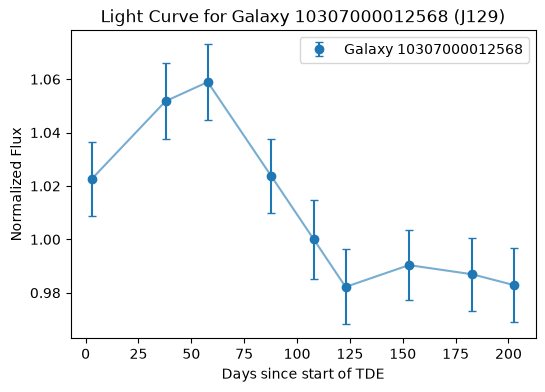
fig_light_curves = plot_multiband_light_curve(host_galaxy, bands, start_mjd=tde_info["start_mjd"])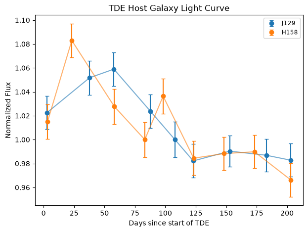
5. Make Cutouts
We follow the example in this tutorial to display cutouts of the potential host galaxies as a function of time with the time listed in the cutout title.
Notebook Cell
def make_cutout(fname, ra, dec, size=100):
    """
    Create a North-up cutout around (RA, Dec) from a Roman TDS FITS image on S3.

    Parameters
    ----------
    fname : str
        Full or partial S3 path to the .fits.gz image.
    ra, dec : float
        Target coordinates in degrees.
    size : int or float, optional
        Cutout size in pixels. Default = 100.

    Returns
    -------
    cutout : astropy.nddata.Cutout2D or None
        Cutout centered on (RA, Dec) and rotated so North points up.
        Returns None if the target is outside the field.
    """

    coord = SkyCoord(ra=ra * u.deg, dec=dec * u.deg)

    with fits.open(fname, fsspec_kwargs={"anon": True}, memmap=False) as hdu:
        img = hdu[1].data
        header = hdu[1].header
        wcs = WCS(header)

        try:
            # Step 1: extract cutout centered on target using the native WCS
            cutout = Cutout2D(img, coord, size, wcs=wcs, mode="partial")
        except Exception as e:
            print(f"Error creating cutout for {fname}: {e}")
            return None
        del img

        # Step 2: determine rotation angle to place North at the top.
        # Invert the CD matrix to find the North direction in pixel space.
        # This handles chip orientation automatically without needing SCA_NUM logic.
        det = header['CD1_1'] * header['CD2_2'] - header['CD1_2'] * header['CD2_1']
        north_col = -header['CD1_2'] / det
        north_row =  header['CD1_1'] / det
        angle = (-np.degrees(np.arctan2(north_col, north_row))) % 360

        # Step 3: rotate only the small cutout (not the full image) to align North up
        cutout.data = rotate(cutout.data, angle=angle, reshape=False, cval=np.nan)

        return cutout
Notebook Cell
def cutout_gallery(image_filenames, mjd_list, ra, dec, aperture_radius_pix_list, size=100, ncols=4,
                   galaxy_id=None):
    """
    Display a gallery of cutouts centered on (RA, Dec) for a list of Roman TDS images.

    Parameters
    ----------
    image_filenames : list of str
        List of S3 image filenames.
    mjd_list : list-like
        Observation MJD values aligned with `image_filenames`.
    ra, dec : float
        Target coordinates in degrees.
    aperture_radius_pix_list : list of float
        Aperture radius values in pixels, aligned with `image_filenames`.
    size : int or float, optional
        Cutout size in pixels. Default = 100.
    ncols : int, optional
        Number of columns in the gallery grid. Default = 4.
    galaxy_id : int or str, optional
        Galaxy ID for labeling the plot.

    Returns
    -------
    fig : matplotlib.figure.Figure
        The displayed figure object.
    """
    # Initialize lists to store image cutouts, observation times, and aligned pixel radii.
    cutouts, mjds, radii_pix = [], [], []

    # Loop over all image filenames and generate cutouts and only keep MJDs and pixel radii for those with valid cutouts
    for fname, mjd, radius_pix in zip(image_filenames, mjd_list, aperture_radius_pix_list):
        cutout = make_cutout(fname, ra, dec, size=size)
        if cutout is not None:
            cutouts.append(cutout)
            mjds.append(mjd)
            radii_pix.append(radius_pix)

    # Stop if no valid cutouts were created
    if not cutouts:
        raise ValueError("No valid cutouts could be created.")

    # Set up grid dimensions for displaying the gallery
    n_images = len(cutouts)
    nrows = int(np.ceil(n_images / ncols))
    fig, axes = plt.subplots(nrows, ncols, figsize=(3 * ncols, 3 * nrows))
    axes = np.atleast_1d(axes).ravel()

    # Build figure title if information is available
    if galaxy_id is not None:
        fig.suptitle(
            f"Cutouts of TDE host galaxy {galaxy_id}",
            fontsize=14, y=0.98
        )
    elif galaxy_id is not None:
        fig.suptitle(
            f"Cutouts for host galaxy {galaxy_id}",
            fontsize=14, y=0.98
        )

    # Display each cutout image with contrast scaling and MJD label
    for ax, cutout, mjd, radius_pix in zip(axes, cutouts, mjds, radii_pix):
        img = cutout.data
        vmin, vmax = np.nanpercentile(img, [5, 99])
        ax.imshow(img, origin="lower", cmap="gray", vmin=vmin, vmax=vmax)
        # Draw the aperture circle at the image center.
        # The galaxy is centered by Cutout2D and stays centered after the North-up rotation.
        x_center = img.shape[1] / 2.0
        y_center = img.shape[0] / 2.0
        if np.isfinite(radius_pix) and radius_pix > 0:
            aperture_circle = plt.Circle((x_center, y_center), radius_pix,
                                         edgecolor="cyan", facecolor="none", linewidth=1.3)
            ax.add_patch(aperture_circle)

        ax.set_title(f"MJD {mjd:.2f}", fontsize=8)
        ax.axis("off")

    # Hide any extra axes
    for ax in axes[len(cutouts):]:
        ax.axis("off")

    plt.tight_layout()
    plt.show()
    return
# make cutout gallery of the host galaxy
# Number of cutout images to display. Increase to show more epochs.
n_cutout_images = 4
single_gal = host_galaxy.iloc[0]
selected_filenames = single_gal[f"image_filenames_{bands[0]}"][:n_cutout_images]
selected_mjds = single_gal[f"mjd_obs_{bands[0]}"][:n_cutout_images]
selected_radius_pix = single_gal["aperture_radius_pix"][:n_cutout_images]
cutout_gallery(
image_filenames=selected_filenames,
mjd_list=selected_mjds,
ra=single_gal["ra"],
dec=single_gal["dec"],
aperture_radius_pix_list=selected_radius_pix,
size=100,
ncols=3,
galaxy_id=single_gal["galaxy_id"],
)
# You may get a `FITSFixedWarning` this is completely harmless and
# just means there is an extra space in the DATE-OBS keyword that astropy is fixing.WARNING: FITSFixedWarning: 'datfix' made the change 'Changed DATE-OBS from '2029-04-04 21:20:09.600000' to '2029-04-04T21:20:09.600000''. [astropy.wcs.wcs]
WARNING: FITSFixedWarning: 'datfix' made the change 'Changed DATE-OBS from '2029-05-09 18:57:36' to '2029-05-09T18:57:36''. [astropy.wcs.wcs]
WARNING: FITSFixedWarning: 'datfix' made the change 'Changed DATE-OBS from '2029-05-29 17:49:55.200000' to '2029-05-29T17:49:55.200000''. [astropy.wcs.wcs]
WARNING: FITSFixedWarning: 'datfix' made the change 'Changed DATE-OBS from '2029-06-28 19:16:19.200000' to '2029-06-28T19:16:19.200000''. [astropy.wcs.wcs]
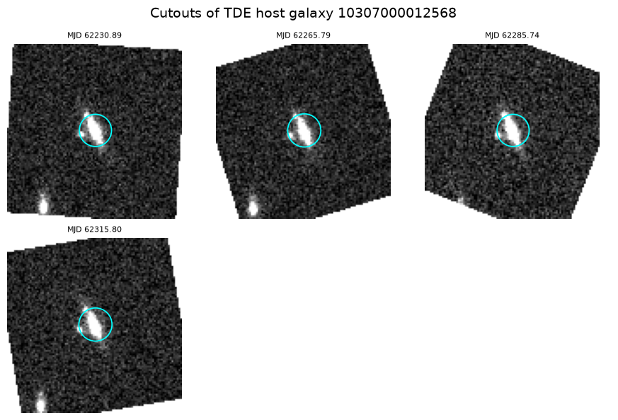
Each cutout is extracted from the larger detector image and then rotated to place North up. The blank regions in the corners are areas outside the original square cutout that become empty after rotation.
Acknowledgements
This work made use of Astropy:\footnote{http://
www .astropy .org} a community-developed core Python package and an ecosystem of tools and resources for astronomy. This research made use of Photutils, an Astropy package for detection and photometry of astronomical sources (Bradley et al. <2025>).
About this notebook
Authors: Jessica Krick, Jaladh Singhal, Brigitta Sipőcz
Updated: 2026-04-02
Contact: IRSA Helpdesk with questions or problems.
Runtime: As of the date above, this notebook takes about 250s to run to completion on a machine with 8GB RAM and 4 CPU.
AI Acknowledgement:
This tutorial was developed with the assistance of AI tools
References:
Bradley et al., 2025; https://
zenodo .org /records /19636730 Virtanen et al., 2020; DOI: 10.1038/s41592-019-0686-2.
- Alarcon, A., Aldoroty, L., Beltz-Mohrmann, G., Bera, A., Blazek, J., Bogart, J., Braeunlich, G., Broughton, A., Cao, K., Chiang, J., Chisari, N. E., Desai, V., Fang, Y., Galbany, L., Hearin, A., Heitmann, K., Hirata, C., Hounsell, R., Jain, B., … Zhang, T. (2025). OpenUniverse2024: a shared, simulated view of the sky for the next generation of cosmological surveys. Monthly Notices of the Royal Astronomical Society, 544(4), 3799–3823. 10.1093/mnras/staf1833