Known Object Name Association (KONA)

Known Object Name Association (KONA), takes a given field of view and computes what objects are contained within it. This is a relatively expensive operation, and is more efficiently done with many images at once, preferably as close together in time as possible.

First we do some setup, including importing many needed packages.

import kete
import matplotlib.pyplot as plt
import numpy as np
import datetime
import warnings

import astropy
from astropy.io import fits
from astropy.wcs import WCS

FITs File

First we load a FITs file, and grab frame information from its header. Observer position is loaded from this file, and the edges of the field of view are calculated from the corners of the frame.

frame = fits.open("data/01772a127-w3-int-1b.fits.gz")[0]

# Here we compute a State of the observer, this could also be constructed
# using spice kernels using kete.spice.state
sc_pos = kete.Vector([frame.header['SUN2SCX'],
                        frame.header['SUN2SCY'],
                        frame.header['SUN2SCZ']],
                    kete.Frames.Equatorial)
sc_vel = kete.Vector([frame.header['SCVELX'],
                        frame.header['SCVELY'],
                        frame.header['SCVELZ']],
                    kete.Frames.Equatorial)

# Load the time
time = datetime.datetime.fromisoformat(frame.header['DATIME'])
# add utc timezone to date
time = time.replace(tzinfo=datetime.timezone.utc)
# now it is correctly formatted, load it
time_jd = kete.Time.from_iso(time.isoformat()).jd

# Now there is a final state of the observer
sc_state = kete.State("WISE", time_jd, sc_pos, sc_vel)


# Build the corner position of the FOV in RA/DEC, and build those into vectors
# The WCS will raise a warning because the FITs files produced by WISE use an
# old format.
with warnings.catch_warnings():
    warnings.filterwarnings("ignore")
    frame_wcs = WCS(frame.header)
corners = []
dx, dy = frame_wcs.pixel_shape
for x, y in zip([0, 0, dx, dx], [0, dy, dy, 0]):
    coord = frame_wcs.pixel_to_world(x, y).icrs
    corners.append(kete.Vector.from_ra_dec(coord.ra.deg, coord.dec.deg))

# Build a generic FOV from the corners and the state of the observer
fov = kete.fov.RectangleFOV.from_corners(corners, sc_state)

MPC Orbit Data

Next we must collect orbit information from the Minor Planet Center (MPC). We will load all known objects from their database, convert them to a kete State, and propagate those states to the epoch near the FITs file epoch we opened.

Note

This takes about 10-15 minutes to run on a powerful desktop, as it is performing orbit propagation using full N-Body mechanics of all planets with corrections for general relativity. This is propagating the entire MPC catalog more than 14 years.

# Load orbit data from the MPC
mpc_obs = kete.mpc.fetch_known_orbit_data()

# Convert that data to State objects.
mpc_states = kete.mpc.table_to_states(mpc_obs)

# It takes a while to propagate 1.5 million asteroids 14 years...
mpc_states = kete.propagate_n_body(mpc_states, time_jd)

Geometry Checks

Calculate what is visible in the frame. Note that this actually accepts any number of frames, and it is strongly recommended to give it all your FOVs of interest at one time. It will be significantly more efficient in its computation. Here we only give it one, and then immediately take the single result back out.

visible_obj = kete.fov_state_check(mpc_states, [fov])[0]

Results

Plot the first n_show=20 objects which were found in the field, but note that 181 known objects have landed in this single FITs frame! That is perhaps unsurprising, as this fits frame is on the ecliptic plane.

n_show = 20
print("Found: ", len(visible_obj))
print(f"Showing top: {n_show}")
print(f"{'Name':<15}{'RA':<15}{'DEC':<15}")
print("-"*45)
for state in list(visible_obj)[:n_show]:
    vec = (state.pos - visible_obj.fov.observer.pos).as_equatorial
    print(f"{state.desig:<15s}{vec.ra_hms:<15s}{vec.dec_dms:<15s}")

Found:  181
Showing top: 20
Name           RA             DEC
---------------------------------------------
          15 13 39.758   -18 50 09.19
         15 14 46.674   -18 19 27.81
         15 14 12.436   -18 44 42.05
        15 13 04.459   -18 56 52.80
        15 14 06.714   -18 51 36.23
        15 14 01.716   -18 18 21.00
        15 13 59.847   -18 50 07.33
        15 13 20.144   -18 45 50.84
        15 14 17.820   -18 44 08.77
        15 13 24.111   -18 39 13.07
        15 14 38.351   -18 35 33.58
        15 14 00.191   -18 39 04.66
        15 14 23.103   -18 51 16.29
        15 13 40.360   -18 53 14.05
        15 13 17.290   -18 56 03.63
        15 15 04.639   -18 54 58.35
        15 13 22.331   -18 29 11.80
        15 13 21.224   -18 16 25.10
100566         15 13 48.365   -18 28 44.76
101066         15 12 44.206   -18 17 42.31

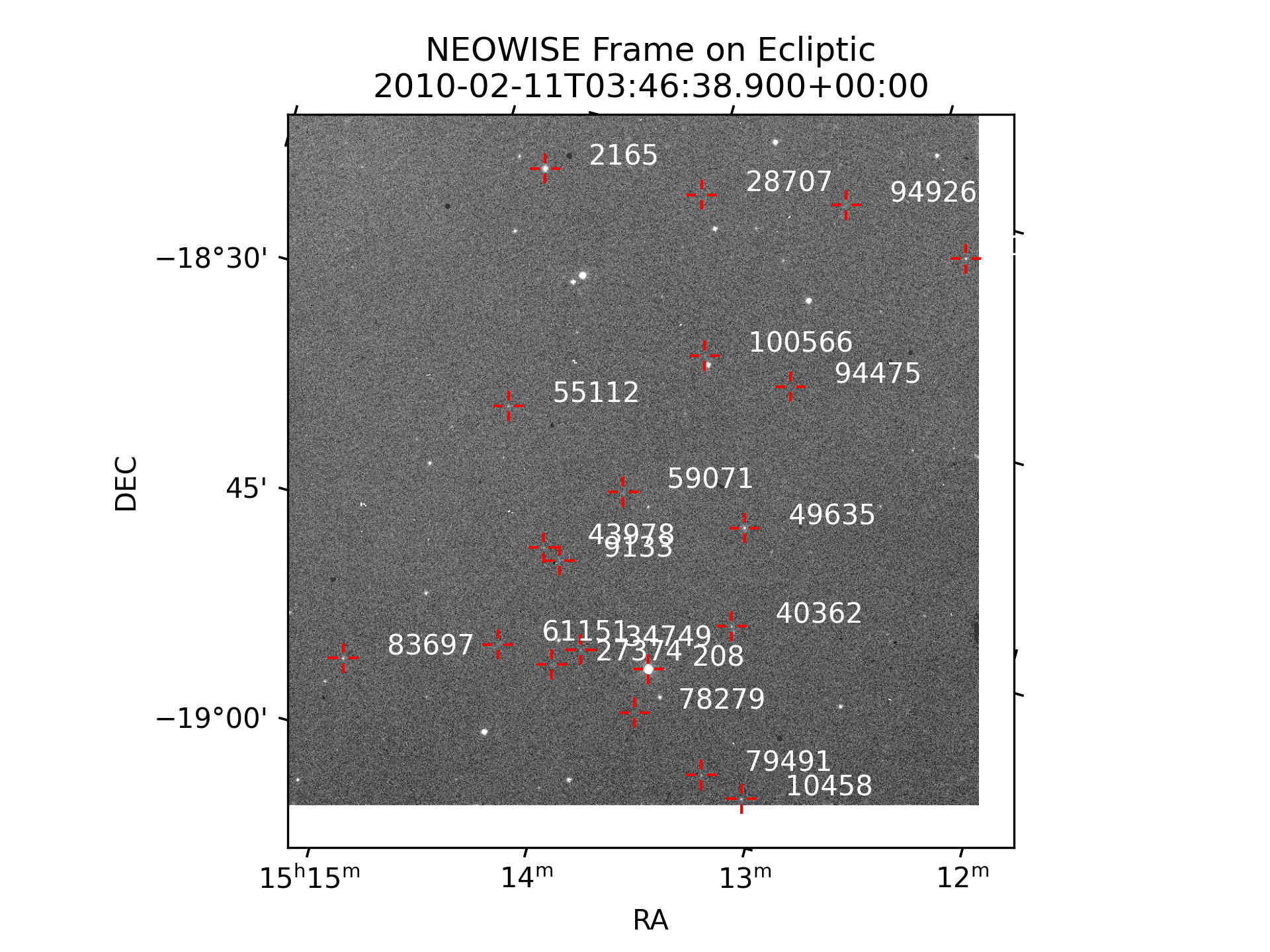
Plotting

Now take the same results from above an plot the fits file with the overlaid positions. Note again this is only showing the first 20 of 181.

plt.figure(dpi=300)
wcs = kete.irsa.plot_fits_image(frame, cmap='grey')
for state in list(visible_obj)[:n_show]:
    vec = (state.pos - visible_obj.fov.observer.pos).as_equatorial
    kete.irsa.annotate_plot(wcs, vec.ra, vec.dec, state.desig, px_gap=10, length=10)
plt.xlabel("RA")
plt.ylabel("DEC")
plt.title(f"NEOWISE Frame on Ecliptic\n{kete.Time(time_jd).iso}");
plt.savefig("data/kona.png")
plt.close()