Palomar 1950 Plate
Identification of an asteroid in a glass plate exposure from 1950 Palomar Mountain.
Background
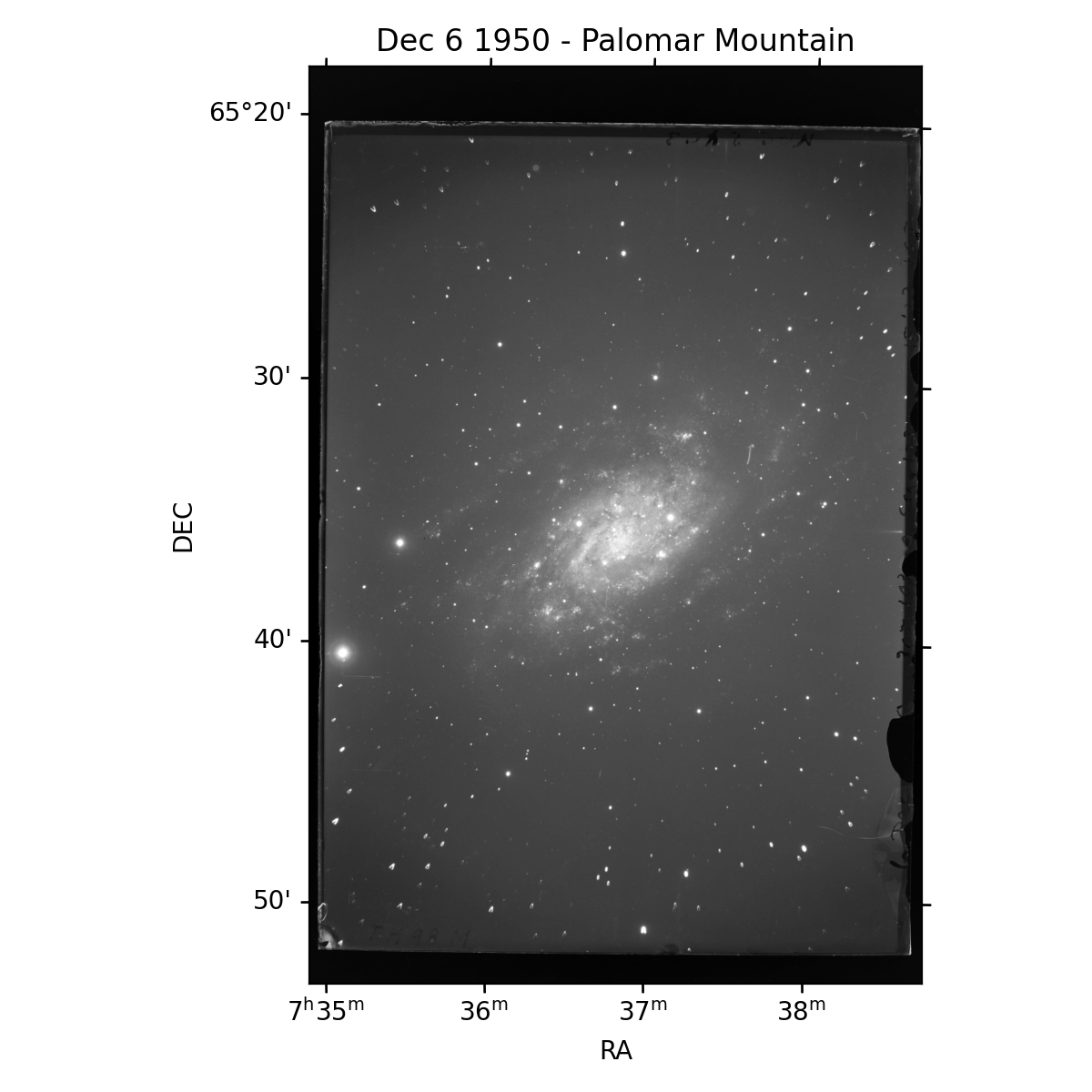
On December 6th and 8th 1950, Rudolph Minkowski captured 2 long exposure images onto glass plates of the galaxy NGC2403 looking for time varying sources. On the cover slip for these plates was written “Asteroid”, and an arrow was drawn on the plate identifying the streaking asteroid on the plates themselves. Details of the observations are included in Tammann & Sandage (1968) in their Table A1, although plate PH-98M is incorrectly listed as PH-98H (with the ending letter indicating the observer). These plates were exposed for approximately 30 minutes (although cloud cover reduced the exposure toward the end for one plate).
These plates are stored at the Carnegie Science Observatories in Pasadena in their archives. One of Carnegie’s Archivists, Kit Whitten, provided a scanned copy of the frames to Joe Masiero at CalTech IPAC around 2018. Masiero provided them for the following analysis.
Here we will identify that asteroid which Minkowski captured over 70 years ago.
Pre-processing
Some pre-processing was done on the scanned image before this analysis. First the data was binned by a factor of 8 in both axis to reduce the file size. Second it was passed to astrometry.net for a plate solution. This gives a valid WCS to work with, which is practically a requirement. Since the image was as scan of a film negative, it was also inverted.
Limitations
Astrometry.net is using the current star catalog, meaning if there are stars in the field which have moved measurably, then the astrometry will be imperfect.
Observer position before 1972 is somewhat tricky to compute, and is currently not well supported in Kete. This is a result of NASA NAIF (Navigation and Ancillary Information Facility) only producing Earth orientation files back to about 1972. This information can be calculated by other means with less precision, but this is not currently implemented. As a result of this, the center of the Earth is used as an approximation for the observers position, but this results in about an arc-minute offset in calculated positions. Adding a better approximation of the observer location shifts the results to sub PSF accuracy.
Record keeping of the exact time appears to be off by a few minutes, though this may be an artifact of the observer position being approximate.
FITs File
First we load a FITs file, and grab frame information from its header.
import kete
import matplotlib.pyplot as plt
import numpy as np

from astropy.io import fits
from astropy.wcs import WCS


# load the fits file and associated WCS
frame = fits.open("data/19501206-NGC2403-reduced.fits.gz")[0]
wcs = WCS(frame.header)

# Time of observation, approximately 3 am local time
# Taken from table A1 of the paper cited above.
jd = kete.Time(2433622.977, scaling='utc').jd

earth = kete.spice.get_state("Earth", jd)
fov = kete.fov.RectangleFOV.from_wcs(wcs, earth)

# Plot the frame
kete.irsa.plot_fits_image(frame)
plt.title("Dec 6 1950 - Palomar Mountain")
plt.tight_layout()
plt.savefig("data/full_frame.png")
MPC Orbit Data
Next we must collect orbit information from the Minor Planet Center (MPC). We will load all known objects from their database, convert them to a kete State, and propagate those states to the epoch near the FITs file epoch we opened.
We also trim out more distant and eccentric objects.
table = kete.mpc.fetch_known_orbit_data()
table = table[[str(t).isdigit() for t in table['desig']]]
table = table[table['ecc'] < 0.5]
table = table[table['peri_dist'] < 4]
states = kete.mpc.table_to_states(table)
Quick Cut
As we are only analyzing a single frame, and the speed of the object suggests it is not close to Earth, we can apply some approximations to remove many objects from contention.
Note
This step below can be completely skipped, it is only an optimization to make the orbit propagation faster. This step only really applies for off ecliptic field of views, as any FOV on the ecliptic will already have most of the main belt as possible objects.
If we assume most objects stay in their orbital plane, but we simply don’t know where they are along the plane, we can use the two body approximation to compute the plane’s on sky position from the observers location.
Here we assume that the object is likely a main belt, or main belt adjacent object, and in doing so we can assume an orbital period of between about 800 and 2500 days.
If we sample the orbit 360 times around the period of 2500 days, objects with that period will be sampled at about 1 degree steps on the sky. We then check at each of these points how close the object came to the center of the FOV.
# Define a convenience function to see how far the objects are from the FOV
def cur_angles(states, fov):
    """
    Given a list of states, compute how far they are from the center of a FOV
    """
    pointing = fov.pointing
    angles = []
    obs_pos = fov.observer.pos
    for state in states:
        vec = state.pos - obs_pos
        angles.append(pointing.angle_between(vec))
    return np.array(angles)

n_steps = 360
period = 2500

jd = np.median([s.jd for s in states])
states = kete.propagate_two_body(states, jd)
best = cur_angles(states, fov)

for dt in np.linspace(0, 1, n_steps) * period:
    states = kete.propagate_two_body(states, jd + dt)
    cur = cur_angles(states, fov)
    best = np.min([best, cur], axis=0)

mask = best < 3
print(f"Total of {sum(mask)} asteroids less than 3 degrees from the FOV")
states = kete.mpc.table_to_states(table[mask])
Total of 1148 asteroids less than 3 degrees from the FOV
Exact Calculation
Compute the visible states, including large main belt asteroids in the computation. For 1k objects this should take about a second.
vis = kete.fov_state_check(states, [fov], include_asteroids=True)[0]
Results
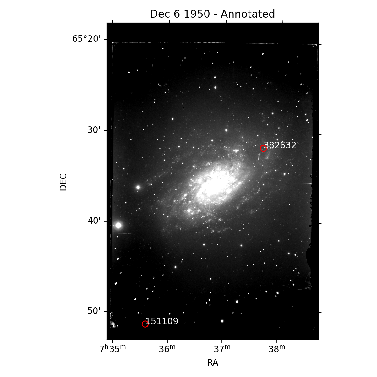
Plot the overlap of visible objects on the original frame.
Two objects are possible, 382632 and 151109, however the second is off the edge of the glass plate itself so not visible.
wcs = kete.irsa.plot_fits_image(frame, percentiles=(40, 99))
for idx in range(len(vis)):
    vec = vis.obs_vecs[idx]
    kete.irsa.annotate_plot(wcs, vec, style='o', px_gap=10, text=vis[idx].desig)

plt.title("Dec 6 1950 - Annotated")
plt.savefig("data/full_frame_annotated.png")
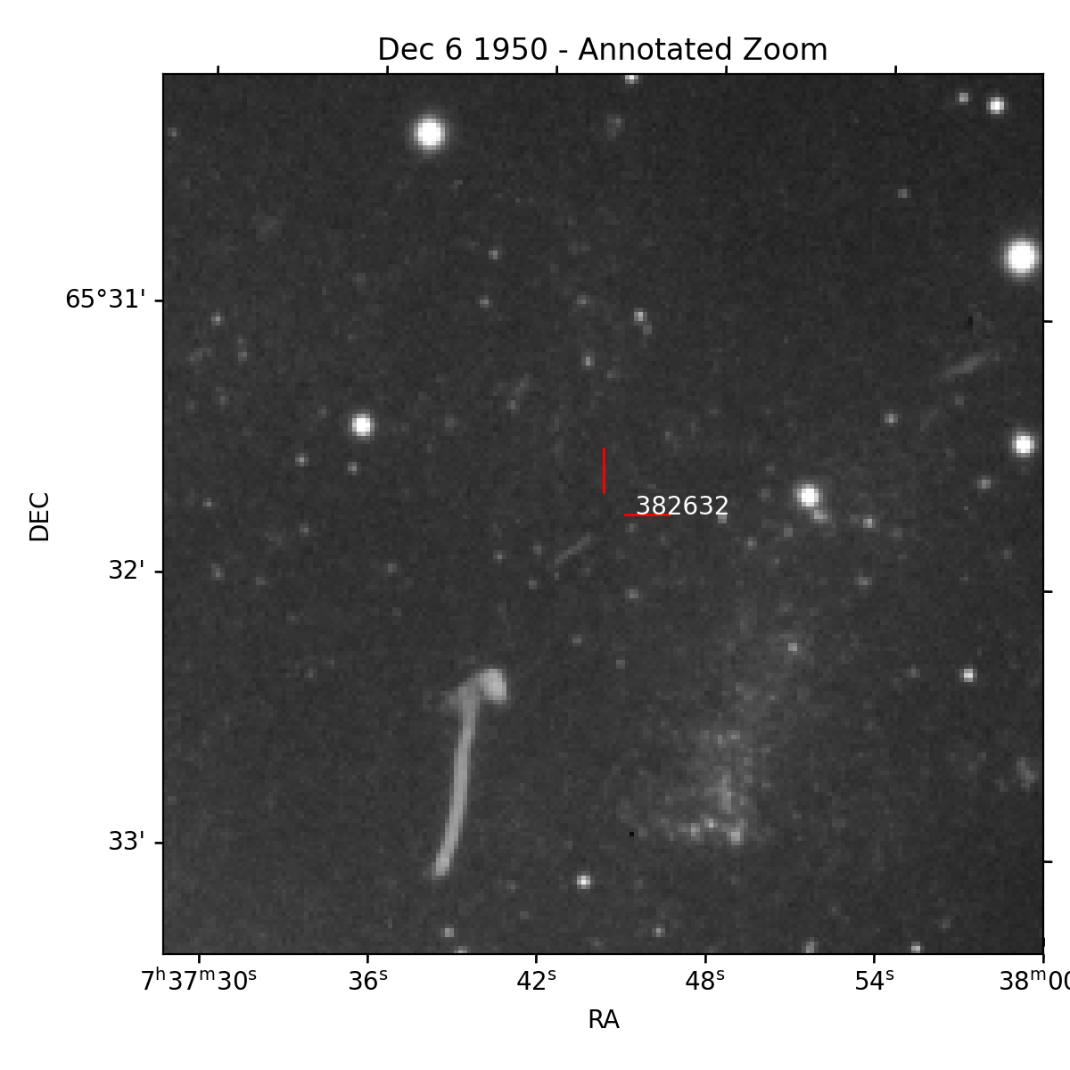
Zoomed
Zooming in to the expected position of 382632, we see the original hand drawn arrow, along with correctly labeled streaking asteroid. Note the slight offset, which from analysis not performed here can be shown to be a result of our assumption that the observer is at the center of the Earth. A better assumption about observer position causes the alignment to match within the width of the blur.
wcs = kete.irsa.plot_fits_image(frame, percentiles=(30, 99.9))
kete.irsa.annotate_plot(wcs,
                        vis.obs_vecs[1],
                        style='L',
                        px_gap=5,
                        length=10,
                        text="    " + vis[1].desig)
kete.irsa.zoom_plot(wcs, vis.obs_vecs[1])
plt.title(f"Dec 6 1950 - Annotated Zoom");
plt.savefig("data/full_frame_annotated_zoom.png")
plt.close()
Higher Resolution
A more precise estimate of the position of Palomar may be approximated using these functions:
def earth_rotation_angle(jd):
    """
    Approximation of Earth Rotation Angle (ERA) with respect to the
    Equatorial J2000 X-Axis.
    """
    jd = kete.Time(jd).utc_jd - 2451545.0
    return (0.779057273264 + 1.0027379094 * jd) * 360

def earth_pos_to_eclip_approx(jd, lat, lon, altitude):
    """
    Given a time and a position on Earth's surface (WGS84 lat/lon and
    altitude in km), approximate the position of this spot on Earth in the
    solar system.

    This is good to within about 1km over a century, however it allows
    us to estimate observer positions before ~1970, where we do not have
    SPICE PCK files. This was validated against the PCK files provided by
    SPICE.
    """

    rotation = np.array(kete.conversion.earth_precession_rotation(jd))
    earth = kete.spice.get_state("Earth", jd).pos.as_equatorial

    era = earth_rotation_angle(jd)

    # Compute the position in ecef
    ecef = kete.vector.wgs_lat_lon_to_ecef(lat, lon, altitude)
    # Rotate this around the earth's current north pole for the fraction of
    # the day
    ecef = np.array(kete.Vector(ecef).rotate_around((0, 0, 1), era))
    # convert the local north to j2000 equatorial north
    eq_ecef = kete.Vector(rotation.T @ ecef, frame=kete.Frames.Equatorial)

    return earth + eq_ecef.as_ecliptic / kete.constants.AU_KM