Euclid Q1: PHZ catalogs#
Learning Goals#
By the end of this tutorial, you will:
Understand the basic characteristics of Euclid Q1 photo-z catalog and how to match it with MER mosaics.
Understand what PHZ catalogs are available and how to view the columns in those catalogs.
How to query with ADQL in the PHZ catalog to find galaxies between a redshift of 1.4 and 1.6.
Pull and plot a spectrum of one of the galaxies in that catalog.
Cutout an image of the galaxy to view it close up.
Learn how to upload images and catalogs to Firefly to inspect individual sources in greater detail.
Introduction#
Euclid launched in July 2023 as a European Space Agency (ESA) mission with involvement by NASA. The primary science goals of Euclid are to better understand the composition and evolution of the dark Universe. The Euclid mission is providing space-based imaging and spectroscopy as well as supporting ground-based imaging to achieve these primary goals. These data will be archived by multiple global repositories, including IRSA, where they will support transformational work in many areas of astrophysics.
Euclid Quick Release 1 (Q1) consists of consists of ~30 TB of imaging, spectroscopy, and catalogs covering four non-contiguous fields: Euclid Deep Field North (22.9 sq deg), Euclid Deep Field Fornax (12.1 sq deg), Euclid Deep Field South (28.1 sq deg), and LDN1641.
Among the data products included in the Q1 release are multiple catalogs created by the PHZ Processing Function. This notebook provides an introduction to the main PHZ catalog, which contains 61 columns describing the photometric redshift probability distribution, fluxes, and classification for each source. If you have questions about this notebook, please contact the IRSA helpdesk.
Imports#
Important
We rely on astroquery features that have been recently added, so please make sure you have version v0.4.10 or newer installed.
# Uncomment the next line to install dependencies if needed.
# !pip install matplotlib 'astropy>=5.3' 'astroquery>=0.4.10' fsspec firefly_client
import os
import re
import urllib

import numpy as np
import matplotlib.pyplot as plt

from astropy.coordinates import SkyCoord
from astropy.io import fits
from astropy.nddata import Cutout2D
from astropy.table import QTable
from astropy import units as u
from astropy.utils.data import download_file
from astropy.visualization import ImageNormalize, PercentileInterval, AsinhStretch, LogStretch, quantity_support
from astropy.wcs import WCS

from firefly_client import FireflyClient
from astroquery.ipac.irsa import Irsa
1. Find the MER Tile ID that corresponds to a given RA and Dec#
In this case, choose random coordinates to show a different MER mosaic image. Search a radius around these coordinates.
ra = 268
dec = 66
search_radius= 10 * u.arcsec

coord = SkyCoord(ra, dec, unit='deg', frame='icrs')
Use IRSA to search for all Euclid data on this target#
This searches specifically in the euclid_DpdMerBksMosaic “collection” which is the MER images and catalogs.
Note
This table lists all MER mosaic images available in this position. These mosaics include the Euclid VIS, Y, J, H images, as well as ground-based telescopes which have been put on the same pixel scale. For more information, see the Euclid documentation at IPAC. We use the facility argument below to query for Euclid images only.
image_table = Irsa.query_sia(pos=(coord, search_radius), collection='euclid_DpdMerBksMosaic', facility='Euclid')
Note that there are various image types are returned as well, we filter out the science images from these:
science_images = image_table[image_table['dataproduct_subtype'] == 'science']
science_images
| s_ra | s_dec | facility_name | instrument_name | dataproduct_subtype | calib_level | dataproduct_type | energy_bandpassname | energy_emband | obs_id | s_resolution | em_min | em_max | em_res_power | proposal_title | access_url | access_format | access_estsize | t_exptime | s_region | obs_collection | obs_intent | algorithm_name | facility_keywords | instrument_keywords | environment_photometric | proposal_id | proposal_pi | proposal_project | target_name | target_type | target_standard | target_moving | target_keywords | obs_release_date | s_xel1 | s_xel2 | s_pixel_scale | position_timedependent | t_min | t_max | t_resolution | t_xel | obs_publisher_did | s_fov | em_xel | pol_states | pol_xel | cloud_access | o_ucd | upload_row_id |
|---|---|---|---|---|---|---|---|---|---|---|---|---|---|---|---|---|---|---|---|---|---|---|---|---|---|---|---|---|---|---|---|---|---|---|---|---|---|---|---|---|---|---|---|---|---|---|---|---|---|---|
| deg | deg | arcsec | m | m | kbyte | s | deg | arcsec | d | d | s | deg | ||||||||||||||||||||||||||||||||||||||
| float64 | float64 | object | object | object | int16 | object | object | object | object | float64 | float64 | float64 | float64 | object | object | object | int64 | float64 | object | object | object | object | object | object | bool | object | object | object | object | object | bool | bool | object | object | int64 | int64 | float64 | bool | float64 | float64 | float64 | int64 | object | float64 | int64 | object | int64 | object | object | int64 |
| 267.66769845285177 | 66.00001388888512 | Euclid | VIS | science | 3 | image | VIS | Optical | 102159190_VIS | 0.16 | 5.5e-07 | 9e-07 | 2.1 | Euclid on-the-fly | https://irsa.ipac.caltech.edu/ibe/data/euclid/q1/MER/102159190/VIS/EUC_MER_BGSUB-MOSAIC-VIS_TILE102159190-6E6EF8_20241025T010045.358775Z_00.00.fits | image/fits | 1474566 | -- | POLYGON ICRS 268.33021981662876 66.26526742211499 267.0051763768436 66.26526712809576 267.01888399697356 65.73197256576843 268.3165136239277 65.73197285251409 268.33021981662876 66.26526742211499 | euclid_DpdMerBksMosaic | SCIENCE | mosaic | -- | field | -- | False | 2025-05-01 00:00:00 | 19200 | 19200 | 0.100000000000008 | False | -- | -- | -- | -- | ivo://irsa.ipac/euclid_DpdMerBksMosaic?102159190_VIS/VIS | 0.533333333333376 | -- | -- | {"aws": {"bucket_name": "nasa-irsa-euclid-q1", "key":"q1/MER/102159190/VIS/EUC_MER_BGSUB-MOSAIC-VIS_TILE102159190-6E6EF8_20241025T010045.358775Z_00.00.fits", "region": "us-east-1"}} | 1 | |||||||||
| 267.66769845285177 | 66.00001388888512 | Euclid | NISP | science | 3 | image | J | Infrared | 102159190_NISP | 0.094 | 1.146e-06 | 1.372e-06 | 5.6 | Euclid on-the-fly | https://irsa.ipac.caltech.edu/ibe/data/euclid/q1/MER/102159190/NISP/EUC_MER_BGSUB-MOSAIC-NIR-J_TILE102159190-466EA5_20241024T213358.873569Z_00.00.fits | image/fits | 1474566 | -- | POLYGON ICRS 268.33021981662876 66.26526742211499 267.0051763768436 66.26526712809576 267.01888399697356 65.73197256576843 268.3165136239277 65.73197285251409 268.33021981662876 66.26526742211499 | euclid_DpdMerBksMosaic | SCIENCE | mosaic | -- | field | -- | False | 2025-05-01 00:00:00 | 19200 | 19200 | 0.100000000000008 | False | -- | -- | -- | -- | ivo://irsa.ipac/euclid_DpdMerBksMosaic?102159190_NISP/J | 0.533333333333376 | -- | -- | {"aws": {"bucket_name": "nasa-irsa-euclid-q1", "key":"q1/MER/102159190/NISP/EUC_MER_BGSUB-MOSAIC-NIR-J_TILE102159190-466EA5_20241024T213358.873569Z_00.00.fits", "region": "us-east-1"}} | 1 | |||||||||
| 267.66769845285177 | 66.00001388888512 | Euclid | NISP | science | 3 | image | H | Infrared | 102159190_NISP | 0.1026 | 1.372e-06 | 2e-06 | 2.7 | Euclid on-the-fly | https://irsa.ipac.caltech.edu/ibe/data/euclid/q1/MER/102159190/NISP/EUC_MER_BGSUB-MOSAIC-NIR-H_TILE102159190-2E0C34_20241024T211805.202819Z_00.00.fits | image/fits | 1474566 | -- | POLYGON ICRS 268.33021981662876 66.26526742211499 267.0051763768436 66.26526712809576 267.01888399697356 65.73197256576843 268.3165136239277 65.73197285251409 268.33021981662876 66.26526742211499 | euclid_DpdMerBksMosaic | SCIENCE | mosaic | -- | field | -- | False | 2025-05-01 00:00:00 | 19200 | 19200 | 0.100000000000008 | False | -- | -- | -- | -- | ivo://irsa.ipac/euclid_DpdMerBksMosaic?102159190_NISP/H | 0.533333333333376 | -- | -- | {"aws": {"bucket_name": "nasa-irsa-euclid-q1", "key":"q1/MER/102159190/NISP/EUC_MER_BGSUB-MOSAIC-NIR-H_TILE102159190-2E0C34_20241024T211805.202819Z_00.00.fits", "region": "us-east-1"}} | 1 | |||||||||
| 267.66769845285177 | 66.00001388888512 | Euclid | NISP | science | 3 | image | Y | Infrared | 102159190_NISP | 0.0878 | 9.2e-07 | 1.146e-06 | 4.6 | Euclid on-the-fly | https://irsa.ipac.caltech.edu/ibe/data/euclid/q1/MER/102159190/NISP/EUC_MER_BGSUB-MOSAIC-NIR-Y_TILE102159190-91C6B0_20241024T212204.431524Z_00.00.fits | image/fits | 1474566 | -- | POLYGON ICRS 268.33021981662876 66.26526742211499 267.0051763768436 66.26526712809576 267.01888399697356 65.73197256576843 268.3165136239277 65.73197285251409 268.33021981662876 66.26526742211499 | euclid_DpdMerBksMosaic | SCIENCE | mosaic | -- | field | -- | False | 2025-05-01 00:00:00 | 19200 | 19200 | 0.100000000000008 | False | -- | -- | -- | -- | ivo://irsa.ipac/euclid_DpdMerBksMosaic?102159190_NISP/Y | 0.533333333333376 | -- | -- | {"aws": {"bucket_name": "nasa-irsa-euclid-q1", "key":"q1/MER/102159190/NISP/EUC_MER_BGSUB-MOSAIC-NIR-Y_TILE102159190-91C6B0_20241024T212204.431524Z_00.00.fits", "region": "us-east-1"}} | 1 |
Choose the VIS image and pull the filename and tileID
filename = science_images[science_images['energy_bandpassname'] == 'VIS']['access_url'][0]
tileID = science_images[science_images['energy_bandpassname'] == 'VIS']['obs_id'][0][:9]

print(f'The MER tile ID for this object is : {tileID}')
The MER tile ID for this object is : 102159190
2. Download PHZ catalog from IRSA#
Use IRSA’s TAP to search catalogs
Irsa.list_catalogs(filter='euclid')
{'euclid.tileid_association_q1': 'Euclid Q1 TILEID to Observation ID Association Table',
 'euclid.objectid_spectrafile_association_q1': 'Euclid Q1 Object ID to Spectral File Association Table',
 'euclid.observation_euclid_q1': 'Euclid Q1 CAOM Observation Table',
 'euclid.plane_euclid_q1': 'Euclid Q1 CAOM Plane Table',
 'euclid.artifact_euclid_q1': 'Euclid Q1 CAOM Artifact Table',
 'euclid_q1_mer_catalogue': 'Euclid Q1 MER Catalog',
 'euclid_q1_mer_morphology': 'Euclid Q1 MER Morphology',
 'euclid_q1_mer_cutouts': 'Euclid Q1 MER Cutouts',
 'euclid_q1_phz_photo_z': 'Euclid Q1 PHZ Photo-z Catalog',
 'euclid_q1_phz_star_sed': 'Euclid Q1 PHZ Star SED Catalog',
 'euclid_q1_phz_galaxy_sed': 'Euclid Q1 PHZ Galaxy SED Catalog',
 'euclid_q1_phz_classification': 'Euclid Q1 PHZ Classification Catalog',
 'euclid_q1_phz_qso_physical_parameters': 'Euclid Q1 PHZ QSO Physical Parameters Catalog',
 'euclid_q1_phz_nir_physical_parameters': 'Euclid Q1 PHZ NIR Physical Parameters Catalog',
 'euclid_q1_phz_star_template': 'Euclid Q1 PHZ Star Template Catalog',
 'euclid_q1_spectro_zcatalog_spe_quality': 'Euclid Q1 SPE Redshift Catalog - Quality',
 'euclid_q1_spectro_zcatalog_spe_classification': 'Euclid Q1 SPE Redshift Catalog - Classification',
 'euclid_q1_spectro_zcatalog_spe_galaxy_candidates': 'Euclid Q1 SPE Redshift Catalog - Galaxy Candidates',
 'euclid_q1_spectro_zcatalog_spe_star_candidates': 'Euclid Q1 SPE Redshift Catalog - Star Candidates',
 'euclid_q1_spectro_zcatalog_spe_qso_candidates': 'Euclid Q1 SPE Redshift Catalog - QSO Candidates',
 'euclid_q1_spe_lines_line_features': 'Euclid Q1 SPE Lines Catalog - Spectral Lines',
 'euclid_q1_spe_lines_continuum_features': 'Euclid Q1 SPE Lines Catalog - Continuum Features',
 'euclid_q1_spe_lines_atomic_indices': 'Euclid Q1 SPE Lines Catalog - Atomic Indices',
 'euclid_q1_spe_lines_molecular_indices': 'Euclid Q1 SPE Lines Catalog - Molecular Indices',
 'euclid_q1_spectro_model_catalog_spe_lines_catalog': 'Euclid Q1 SPE Models Catalog - Lines',
 'euclid_q1_spectro_model_catalog_spe_star_models': 'Euclid Q1 SPE Star Models Catalog'}
table_mer = 'euclid_q1_mer_catalogue'
table_phz = 'euclid_q1_phz_photo_z'
table_1dspectra = 'euclid.objectid_spectrafile_association_q1'
Learn some information about the photo-z catalog:#
How many columns are there?
List the column names
columns_info = Irsa.list_columns(catalog=table_phz)
print(len(columns_info))
67
Tip
The PHZ catalog contains 67 columns, below are a few highlights:
object_id
flux_vis_unif, flux_y_unif, flux_j_unif, flux_h_unif
median redshift (phz_median)
phz_classification
phz_90_int1, phz_90_int2 (The phz PDF interval containing 90% of the probability, upper and lower values)
# Full list of columns and their description
columns_info
{'object_id': 'Unique ID of the object in the survey, as set by MER',
 'phz_median': 'The median of the PHZ PDF',
 'phz_mode_1': 'The first mode of the PHZ PDF',
 'phz_mode_1_area': 'The total area of the first mode',
 'phz_mode_2': 'The second mode of the PHZ PDF',
 'phz_mode_2_area': 'The total area of the second mode',
 'bias_id': 'The identifier to be used for retrieving the bias correction shift from the bias correction map',
 'tom_bin_id': 'The identifier of the tomographic bin the source belongs to (Equipopulated-bins)',
 'alt_tom_bin_id': 'The identifier of the alternate tomographic bin the source belongs to (Equidistant-bins)',
 'pos_tom_bin_id': 'The identifier of the photometric clustering tomographic bin the source belongs to (Equipopulated-bins)',
 'flag_som_tomobin': 'Flag telling if the source belong to a combination of SOM cell and Tom. bin which can be calibrated (=1) or not (=0).',
 'flag_som_alt_tomobin': 'Flag telling if the source belong to a combination of SOM cell and Alt Tom. bin which can be calibrated (=1) or not (=0).',
 'flag_som_pos_tomobin': 'Flag telling if the source belong to a combination of SOM cell and POS Tom. bin which can be calibrated (=1) or not (=0).',
 'flux_u_ext_decam_unif': 'Unified flux recomputed after correction from galactic extinction and filter shifts',
 'flux_g_ext_decam_unif': '',
 'flux_r_ext_decam_unif': '',
 'flux_i_ext_decam_unif': '',
 'flux_z_ext_decam_unif': '',
 'flux_u_ext_lsst_unif': '',
 'flux_g_ext_lsst_unif': '',
 'flux_r_ext_lsst_unif': '',
 'flux_i_ext_lsst_unif': '',
 'flux_z_ext_lsst_unif': '',
 'flux_u_ext_megacam_unif': '',
 'flux_g_ext_hsc_unif': '',
 'flux_r_ext_megacam_unif': '',
 'flux_i_ext_panstarrs_unif': '',
 'flux_z_ext_hsc_unif': '',
 'flux_vis_unif': '',
 'flux_y_unif': '',
 'flux_j_unif': '',
 'flux_h_unif': '',
 'fluxerr_u_ext_decam_unif': '',
 'fluxerr_g_ext_decam_unif': '',
 'fluxerr_r_ext_decam_unif': '',
 'fluxerr_i_ext_decam_unif': '',
 'fluxerr_z_ext_decam_unif': '',
 'fluxerr_u_ext_lsst_unif': '',
 'fluxerr_g_ext_lsst_unif': '',
 'fluxerr_r_ext_lsst_unif': '',
 'fluxerr_i_ext_lsst_unif': '',
 'fluxerr_z_ext_lsst_unif': '',
 'fluxerr_u_ext_megacam_unif': '',
 'fluxerr_g_ext_hsc_unif': '',
 'fluxerr_r_ext_megacam_unif': '',
 'fluxerr_i_ext_panstarrs_unif': '',
 'fluxerr_z_ext_hsc_unif': '',
 'fluxerr_vis_unif': '',
 'fluxerr_y_unif': '',
 'fluxerr_j_unif': '',
 'fluxerr_h_unif': '',
 'photometric_system': 'Encode the Photometric band configuration (indicating also the number of missing columns)',
 'phz_classification': 'Classification flag: 1 if the source is accepted as star, 2 if it is accepted as a galaxy, 4 if it is accepted as a QSO, 8 if the source is acce..."',
 'phz_flags': 'An integer containing the flags of the PHZ processing. Meaning: 0 => OK, 1 => NNPZ flag: no close neighbor, 10 not VIS detected, 11 missing band, 12 t...',
 'phz_weight': 'Probability to be a usable source at VIS MAG=23.5',
 'best_chi2': 'Chi2 of the best fit model or the closest neighbor',
 'phz_70_int1': 'The smallest PHZ PDF interval containing 70% of the probability - lower value',
 'phz_70_int2': 'The smallest PHZ PDF interval containing 70% of the probability - upper value',
 'phz_90_int1': 'The smallest PHZ PDF interval containing 90% of the probability - lower value',
 'phz_90_int2': 'The smallest PHZ PDF interval containing 90% of the probability - upper value',
 'phz_95_int1': 'The smallest PHZ PDF interval containing 95% of the probability - upper value',
 'phz_95_int2': '',
 'ie_cuts_weights1': 'Vector of probability to be a usable source for VIS MAG cut 20.25',
 'ie_cuts_weights2': 'Vector of probability to be a usable source for VIS MAG cut 21.25',
 'ie_cuts_weights3': 'Vector of probability to be a usable source for VIS MAG cut 22.25',
 'ie_cuts_weights4': 'Vector of probability to be a usable source for VIS MAG cut 24.5',
 'cntr': 'entry counter (key) number (unique within table)'}
Note
The phz_catalog on IRSA has more columns than it does on the ESA archive. This is because the ESA catalog stores some information in one column (for example, phz_90_int is stored as [lower, upper], rather than in two separate columns).
The fluxes are different from the fluxes derived in the MER catalog. The _unif fluxes are: “Unified flux recomputed after correction from galactic extinction and filter shifts”.
Find some galaxies between 1.4 and 1.6 at a selected RA and Dec#
We specify the following conditions on our search:
We select just the galaxies where the flux is greater than zero, to ensure the appear in all four of the Euclid MER images.
Select only objects in a circle (search radius selected below) around our selected RA and Dec
phz_classification = 2means we select only galaxiesUsing the
phz_90_int1andphz_90_int2, we select just the galaxies where the error on the photometric redshift is less than 20%Select just the galaxies between a median redshift of 1.4 and 1.6
We search just a 5 arcminute box around an RA and Dec
Search based on tileID:
######################## User defined section ############################
## How large do you want the image cutout to be?
im_cutout= 5 * u.arcmin

## What is the center of the cutout?
ra_cutout = 267.8
dec_cutout =  66

coords_cutout = SkyCoord(ra_cutout, dec_cutout, unit='deg', frame='icrs')
size_cutout = im_cutout.to(u.deg).value
adql = ("SELECT DISTINCT mer.object_id, mer.ra, mer.dec, "
        "phz.flux_vis_unif, phz.flux_y_unif, phz.flux_j_unif, phz.flux_h_unif, "
        "phz.phz_classification, phz.phz_median, phz.phz_90_int1, phz.phz_90_int2 "
        f"FROM {table_mer} AS mer "
        f"JOIN {table_phz} as phz "
        "ON mer.object_id = phz.object_id "
        "WHERE 1 = CONTAINS(POINT('ICRS', mer.ra, mer.dec), "
                            f"BOX('ICRS', {ra_cutout}, {dec_cutout}, {size_cutout/np.cos(coords_cutout.dec)}, {size_cutout})) "
        "AND phz.flux_vis_unif> 0 "
        "AND  phz.flux_y_unif > 0 "
        "AND phz.flux_j_unif > 0 "
        "AND phz.flux_h_unif > 0 "
        "AND phz.phz_classification = 2 "
        "AND ((phz.phz_90_int2 - phz.phz_90_int1) / (1 + phz.phz_median)) < 0.20 "
        "AND phz.phz_median BETWEEN 1.4 AND 1.6")


## Use TAP with this ADQL string
result_galaxies = Irsa.query_tap(adql).to_table()
result_galaxies[:5]
| object_id | ra | dec | flux_vis_unif | flux_y_unif | flux_j_unif | flux_h_unif | phz_classification | phz_median | phz_90_int1 | phz_90_int2 |
|---|---|---|---|---|---|---|---|---|---|---|
| deg | deg | uJy | uJy | uJy | uJy | |||||
| int64 | float64 | float64 | float64 | float64 | float64 | float64 | int64 | float32 | float32 | float32 |
| 2678009942660367473 | 267.80099422 | 66.03674732 | 0.7179743124 | 2.652854347 | 3.846100812 | 5.242284889 | 2 | 1.519999981 | 1.350000024 | 1.75 |
| 2678076394659719061 | 267.80763944 | 65.97190620 | 1.432410411 | 3.936189211 | 4.907444279 | 6.222690821 | 2 | 1.600000024 | 1.480000019 | 1.820000052 |
| 2677585153659610182 | 267.75851534 | 65.96101826 | 0.9337781689 | 3.119727456 | 3.711064298 | 4.959729567 | 2 | 1.5 | 1.379999995 | 1.710000038 |
| 2678000211660381851 | 267.80002116 | 66.03818515 | 1.05509166 | 2.605535558 | 3.240129863 | 3.793176892 | 2 | 1.600000024 | 1.470000029 | 1.889999986 |
| 2678361447659819278 | 267.83614472 | 65.98192782 | 1.99473143 | 4.426665941 | 5.28416351 | 6.400697455 | 2 | 1.519999981 | 1.429999948 | 1.850000024 |
Warning
Note that we use to_table above rather than to_qtable. While astropy’s QTable is more powerful than its Table, as it e.g. handles the column units properly, we cannot use it here due to a known bug; it mishandles the large integer numbers in the object_id column and recast them as float during which process some precision is being lost.
Once the bug is fixed, we plan to update the code in this notebook and simplify some of the approaches below.
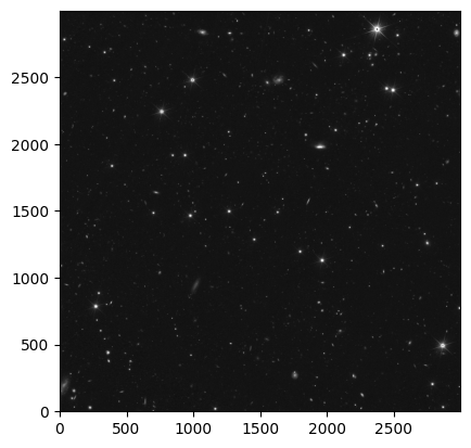
3. Read in a cutout of the MER image from IRSA directly#
Due to the large field of view of the MER mosaic, let’s cut out a smaller section (5’x5’) of the MER mosaic to inspect the image.
## Use fsspec to interact with the fits file without downloading the full file
hdu = fits.open(filename, use_fsspec=True)

## Store the header
header = hdu[0].header

## Read in the cutout of the image that you want
cutout_image = Cutout2D(hdu[0].section, position=coords_cutout, size=im_cutout, wcs=WCS(header))
cutout_image.data.shape
(3000, 3000)
norm = ImageNormalize(cutout_image.data, interval=PercentileInterval(99.9), stretch=AsinhStretch())
_ = plt.imshow(cutout_image.data, cmap='gray', origin='lower', norm=norm)
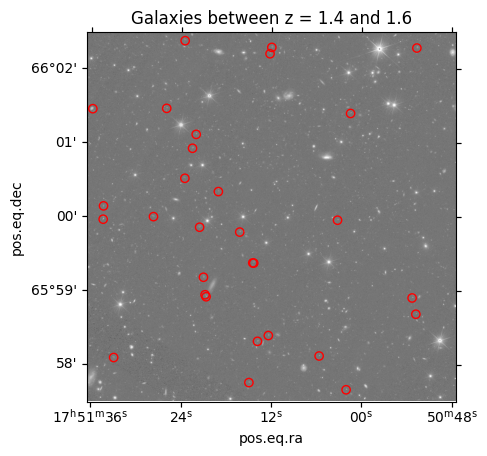
4. Overplot the catalog on the MER mosaic image#
Tip
We can rely on astropy’s WCSAxes framework for making plots of Astronomical data in Matplotlib. Please note the usage of projection and transform arguments in the code example below.
For more info, please visit the WCSAxes documentation.
ax = plt.subplot(projection=cutout_image.wcs)

ax.imshow(cutout_image.data, cmap='gray', origin='lower',
          norm=ImageNormalize(cutout_image.data, interval=PercentileInterval(99.9), stretch=LogStretch()))
plt.scatter(result_galaxies['ra'], result_galaxies['dec'], s=36, facecolors='none', edgecolors='red',
            transform=ax.get_transform('world'))

_ = plt.title('Galaxies between z = 1.4 and 1.6')
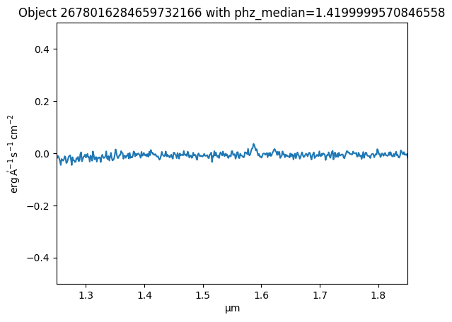
5. Pull the spectra on the top brightest source based on object ID#
result_galaxies.sort(keys='flux_h_unif', reverse=True)
result_galaxies[:3]
| object_id | ra | dec | flux_vis_unif | flux_y_unif | flux_j_unif | flux_h_unif | phz_classification | phz_median | phz_90_int1 | phz_90_int2 |
|---|---|---|---|---|---|---|---|---|---|---|
| deg | deg | uJy | uJy | uJy | uJy | |||||
| int64 | float64 | float64 | float64 | float64 | float64 | float64 | int64 | float32 | float32 | float32 |
| 2677562455660233171 | 267.75624552 | 66.02331715 | 0.9376629547 | 6.932368948 | 13.77487169 | 18.16076037 | 2 | 1.419999957 | 1.309999943 | 1.549999952 |
| 2678376290659863203 | 267.83762908 | 65.98632035 | 1.795682573 | 6.656510568 | 8.965489634 | 12.90360126 | 2 | 1.539999962 | 1.49000001 | 1.610000014 |
| 2678016284659732166 | 267.80162845 | 65.97321669 | 1.291915237 | 5.271049845 | 7.114689858 | 10.88637487 | 2 | 1.419999957 | 1.25999999 | 1.480000019 |
Let’s pick one of these galaxies. Note that the table has been sorted above, we can use the same index here and below to access the data for this particular galaxy.
index = 2

obj_id = result_galaxies['object_id'][index]
redshift = result_galaxies['phz_median'][index]
We will use TAP and an ASQL query to find the spectral data for this particular galaxy.
adql_object = f"SELECT * FROM {table_1dspectra} WHERE objectid = {obj_id}"

## Pull the data on this particular galaxy
result_spectra = Irsa.query_tap(adql_object).to_table()
result_spectra
| objectid | tileid | uri | hdu | cntr |
|---|---|---|---|---|
| int64 | int64 | object | int64 | int64 |
| 2678016284659732166 | 102159190 | ibe/data/euclid/q1/SIR/102159190/EUC_SIR_W-COMBSPEC_102159190_2024-11-05T16:14:02.114614Z.fits | 1525 | 59948 |
Pull out the file name from the result_spectra table:
file_uri = urllib.parse.urljoin(Irsa.tap_url, result_spectra['uri'][0])
file_uri
'https://irsa.ipac.caltech.edu/ibe/data/euclid/q1/SIR/102159190/EUC_SIR_W-COMBSPEC_102159190_2024-11-05T16:14:02.114614Z.fits'
with fits.open(file_uri) as hdul:
    spectrum = QTable.read(hdul[result_spectra['hdu'][0]], format='fits')
    spectrum_header = hdul[result_spectra['hdu'][0]].header
WARNING: UnitsWarning: 'Number' did not parse as fits unit: At col 0, Unit 'Number' not supported by the FITS standard.  If this is meant to be a custom unit, define it with 'u.def_unit'. To have it recognized inside a file reader or other code, enable it with 'u.add_enabled_units'. For details, see https://docs.astropy.org/en/latest/units/combining_and_defining.html [astropy.units.core]
WARNING: UnitsWarning: 'Number' did not parse as fits unit: At col 0, Unit 'Number' not supported by the FITS standard.  If this is meant to be a custom unit, define it with 'u.def_unit'. To have it recognized inside a file reader or other code, enable it with 'u.add_enabled_units'. For details, see https://docs.astropy.org/en/latest/units/combining_and_defining.html [astropy.units.core]
WARNING: UnitsWarning: 'Number' did not parse as fits unit: At col 0, Unit 'Number' not supported by the FITS standard.  If this is meant to be a custom unit, define it with 'u.def_unit'. To have it recognized inside a file reader or other code, enable it with 'u.add_enabled_units'. For details, see https://docs.astropy.org/en/latest/units/combining_and_defining.html [astropy.units.core]
Now the data are read in, plot the spectrum#
Tip
As we use astropy.visualization’s quantity_support, matplotlib automatically picks up the axis units from the quantitites we plot.
quantity_support()
<astropy.visualization.units.quantity_support.<locals>.MplQuantityConverter at 0x7f201706bc90>
plt.plot(spectrum['WAVELENGTH'].to(u.micron), spectrum['SIGNAL'])

plt.xlim(1.25, 1.85)
plt.ylim(-0.5, 0.5)
_ = plt.title(f"Object {obj_id} with phz_median={redshift}")
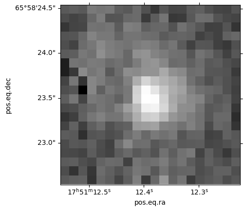
Let’s cut out a very small patch of the MER image to see what this galaxy looks like. Remember that we sorted the table above, so can reuse the same index to pick up the coordinates for the galaxy. Otherwise we could filter on the object ID.
result_galaxies[index]
| object_id | ra | dec | flux_vis_unif | flux_y_unif | flux_j_unif | flux_h_unif | phz_classification | phz_median | phz_90_int1 | phz_90_int2 |
|---|---|---|---|---|---|---|---|---|---|---|
| deg | deg | uJy | uJy | uJy | uJy | |||||
| int64 | float64 | float64 | float64 | float64 | float64 | float64 | int64 | float32 | float32 | float32 |
| 2678016284659732166 | 267.80162845 | 65.97321669 | 1.291915237 | 5.271049845 | 7.114689858 | 10.88637487 | 2 | 1.419999957 | 1.25999999 | 1.480000019 |
## How large do you want the image cutout to be?
size_galaxy_cutout = 2.0 * u.arcsec
Use the ra and dec columns for the galaxy to create a SkyCoord.
coords_galaxy = SkyCoord(result_galaxies['ra'][index], result_galaxies['dec'][index], unit='deg')
coords_galaxy
<SkyCoord (ICRS): (ra, dec) in deg
    (267.80162845, 65.97321669)>
We haven’t closed the image file above, so use Cutout2D again to cut out a section around the galaxy.
cutout_galaxy = Cutout2D(hdu[0].section, position=coords_galaxy, size=size_galaxy_cutout, wcs=WCS(header))
Plot to show the cutout on the galaxy
ax = plt.subplot(projection=cutout_galaxy.wcs)

ax.imshow(cutout_galaxy.data, cmap='gray', origin='lower',
          norm=ImageNormalize(cutout_galaxy.data, interval=PercentileInterval(99.9), stretch=AsinhStretch()))
<matplotlib.image.AxesImage at 0x7f204c54db10>
6. Load the image on Firefly to be able to interact with the data directly#
Save the data locally if you have not already done so, in order to upload to IRSA viewer.
download_path = "data"
if os.path.exists(download_path):
    print("Output directory already created.")
else:
    print("Creating data directory.")
    os.mkdir(download_path)
Creating data directory.
Vizualize the image with Firefly#
First initialize the client, then set the path to the image, upload it to firefly, load it and align with WCS.
Note this can take a while to upload the full MER image.
fc = FireflyClient.make_client('https://irsa.ipac.caltech.edu/irsaviewer')

fc.show_fits(url=filename)

fc.align_images(lock_match=True)
{'success': True}
Save the table as a CSV for Firefly upload#
csv_path = os.path.join(download_path, "mer_df.csv")
result_galaxies.write(csv_path, format="csv")
Upload the CSV table to Firefly and display as an overlay on the FITS image#
uploaded_table = fc.upload_file(csv_path)
print(f"Uploaded Table URL: {uploaded_table}")

fc.show_table(uploaded_table)
Uploaded Table URL: ${upload-dir}/upload_13551808110088607665_mer_df.csv
{'success': True}
About this Notebook#
Author: Tiffany Meshkat, Anahita Alavi, Anastasia Laity, Andreas Faisst, Brigitta Sipőcz, Dan Masters, Harry Teplitz, Jaladh Singhal, Shoubaneh Hemmati, Vandana Desai
Updated: 2025-04-10
Contact: the IRSA Helpdesk with questions or reporting problems.