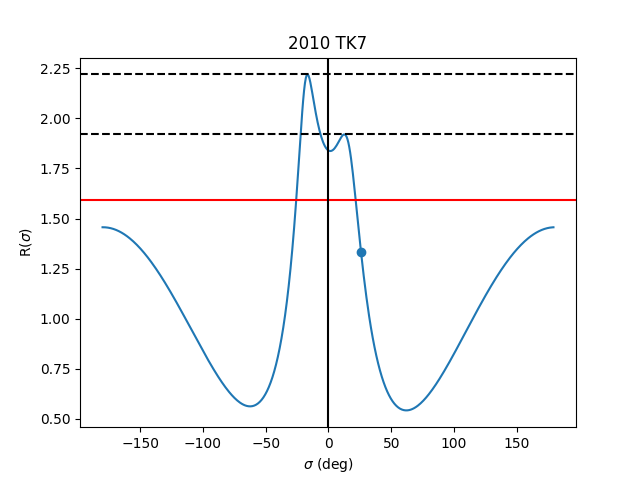
Earth Trojan 2010 TK7

Following some of the analysis from the following papers:

• “2002 AA29: Earth’s recurrent quasi-satellite?” - Paweł Wajer - Icarus - 2009

• “Dynamical evolution of Earth’s quasi-satellites: 2004 GU9 and 2006 FV35” - Paweł Wajer - Icarus - 2010

We can perform some dynamical analysis to see if the asteroid 2010 TK7 appears to be an Earth trojan.

The end result of this is a plot which shows the current energy level of the orbit, if the current position of the object is in a gravitational “low”, and the energy line (in red) is below the height of the walls of that low point, then the object is at least temporarily captured.

import numpy as np
import matplotlib.pyplot as plt
import kete


# Grab 2010 TK7 and propagate it to 2010
state_a = kete.HorizonsProperties.fetch("2010 TK7", update_name=False).state
state_a = kete.propagate_n_body([state_a], kete.Time.from_ymd(2010, 1, 1))[0]

state_b = kete.spice.get_state("Earth", state_a.jd)
# Earth mass in Solar masses
mass_planet = 3.0435727639549377e-06

# n_sigma is the number of step on the x axis in the final plot
n_sigma = 500

# m_steps is the number of steps in the numerical integration
m_steps = 100


jd = state_a.jd

elem_a = state_a.elements
elem_b = state_b.elements

period_a = elem_a.orbital_period
period_b = elem_b.orbital_period

sigma_steps = np.linspace(0, 1, n_sigma + 1)[:-1]

energy_vals = []
for shift in sigma_steps:

    total = 0
    for frac in np.linspace(0, 1, m_steps + 1)[:-1]:
        state_a = kete.propagate_two_body([state_a], jd + (frac + shift) * period_a)[0]
        state_b = kete.propagate_two_body([state_b], jd + frac * period_b)[0]
        pos_a = state_a.pos
        pos_b = state_b.pos
        total += 1 / (pos_b - pos_a).r - np.dot(pos_b, pos_a) / pos_b.r**3

    energy_vals.append(total / m_steps)

cur_energy = (
    3 * (elem_a.semi_major - elem_b.semi_major) ** 2 / (8.0 * mass_planet)
    + energy_vals[0]
)

# energy vals start from the current positions and go a full orbit.
# These may be unrolled so that the Earth is in the middle, the following
# is a series of index manipulations to find the correct position for that.

longitude_b = elem_b.mean_anomaly + elem_b.peri_arg + elem_b.lon_of_ascending
longitude_a = elem_a.mean_anomaly + elem_a.peri_arg + elem_a.lon_of_ascending
i = np.digitize(((longitude_a - longitude_b) % 360) / 360, sigma_steps)

# here are the unrolled values, which may be plotted
vals_unrolled = np.roll(energy_vals, i + n_sigma // 2)
x_unrolled = np.linspace(-180, 180, n_sigma + 1)[:-1]

# plot the energy curve
plt.plot(x_unrolled, vals_unrolled)

# plot the current position of the object
plt.scatter(x_unrolled[(i + n_sigma // 2) % (n_sigma)], energy_vals[0])

# plot the current energy of the object
plt.axhline(cur_energy, c="r")
plt.axvline(0, c="k")

# We can then find and plot the inflection points
local_max = np.argwhere(np.diff(np.sign(np.diff(vals_unrolled))) < 0).ravel() + 1
for x in vals_unrolled[local_max]:
    plt.axhline(x, c="k", ls="--")


plt.xlabel(r"$\sigma$ (deg)")
plt.ylabel(r"R($\sigma)$")
plt.title(f"{elem_a.desig}")
plt.show()