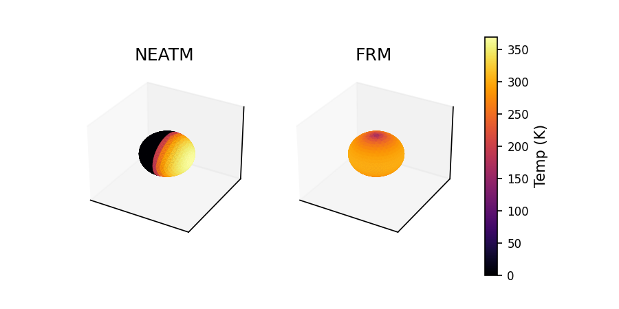
Thermal Model

Visualization of FRM and NEATM thermal models, this computes the temperatures of each part of a spherical asteroid in both models, and plots the results. The geometry is such that the sun is 1 AU away from the asteroid along the X-axis.

import kete
import numpy as np
import matplotlib as mpl
import matplotlib.cm as cm
from mpl_toolkits.mplot3d.art3d import Poly3DCollection
import matplotlib.pyplot as plt

# Compute the temperatures of each facet of an object and plot it in 3d
# Set the physical parameters used for the simulation
g_phase = 0.15
emissivity = 0.9
vis_albedo = 0.05

# Beaming is only used by NEATM
beaming = 1.4

# Define the geometry
geom = kete.shape.TriangleEllipsoid(12)
obj2sun = np.array([1, 0, 0])
# Note: The TriangleEllipsoid geometry is not used by default in the kete code.
# This is because its facet normals tend to be slightly correlated with one another.
# These correlations can be eliminated by setting the number of facets high enough,
# but for a low facet count, the FibonacciLattice converges to the exact answer
# in far fewer total facets. Unfortunately, the FibonacciLattice doesn't have a nice
# geometric representation, meaning it is highly non-trivial to plot, and as a
# result is not used in this example.

# Compute the temperature at the subsolar point on the object.
# Note that FRM uses a beaming = pi
neatm_subsolar_temp = kete.flux.sub_solar_temperature(
    -obj2sun, vis_albedo, g_phase, emissivity, beaming
)
frm_subsolar_temp = kete.flux.sub_solar_temperature(
    -obj2sun, vis_albedo, g_phase, emissivity
)

# Compute the FRM and NEATM facet temperatures for the object
neatm_facet_temps = kete.flux.neatm_facet_temps(
    geom.normals,
    neatm_subsolar_temp,
    obj2sun,
)
frm_facet_temps = kete.flux.frm_facet_temps(
    geom.normals,
    frm_subsolar_temp,
    obj2sun,
)

# Plot the results
plt.figure(dpi=150, figsize=(6, 3))
plt.subplot(121, projection="3d")

norm = mpl.colors.Normalize(vmin=0, vmax=max(neatm_facet_temps))
m = cm.ScalarMappable(norm=norm, cmap=mpl.colormaps["RdBu_r"])
colors = m.to_rgba(neatm_facet_temps, alpha=1)
polygons = Poly3DCollection(geom.facets, edgecolor="black", lw=0.2, color=colors)
plt.gca().add_collection3d(polygons)
plt.xlim(-2, 2)
plt.ylim(-2, 2)
plt.gca().set_zlim(-2, 2)
plt.gca().set_xticks([])
plt.gca().set_yticks([])
plt.gca().set_zticks([])
plt.title("NEATM")

plt.subplot(122, projection="3d")
colors = m.to_rgba(frm_facet_temps, alpha=1)
polygons = Poly3DCollection(geom.facets, edgecolor="black", lw=0.2, color=colors)
plt.gca().add_collection3d(polygons)
plt.xlim(-2, 2)
plt.ylim(-2, 2)
plt.gca().set_zlim(-2, 2)
plt.gca().set_xticks([])
plt.gca().set_yticks([])
plt.gca().set_zticks([])
plt.title("FRM")

cbar = plt.colorbar(m, ax=plt.gcf().axes, label="Temp (K)")
cbar.ax.tick_params(labelsize=8)
plt.show()