Solar Spectrum

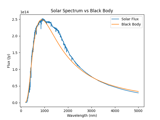
Plot the true Solar spectrum vs a black body approximation.

import kete
import numpy as np
import matplotlib.pyplot as plt

# Sample wavelengths from 200nm to 5um at 1000 points
wavelengths = np.linspace(200, 5000, 1000)

# In units of au
dist_from_sun = 1.0

Reference Solar Spectrum

This is the 2000 ASTM Standard Extraterrestrial Spectrum Reference E-490-00: https://www.nrel.gov/grid/solar-resource/spectra-astm-e490.html

solar_flux = [kete.flux.solar_flux(dist_from_sun, w) for w in wavelengths]

Black Body

Compute black body for the sun from base principles.

sun_r_au = kete.constants.SUN_RADIUS_M / kete.constants.AU_M

# black body radiation is Janskys / steradian, it needs to be integrated over the
# steradian.
black_body_flux = np.array(
    [
        kete.flux.black_body_flux(
            temp=kete.constants.SUN_TEMP,
            wavelength=w,
        )
        for w in wavelengths
    ]
)

# Black body approximation of the solar flux at the radius of where the object is,
# this treats the sun as a flat disk facing the object. This is an approximation
# which breaks down when the object gets within a few solar radii.
sun_black_body_flux = np.pi * black_body_flux * (sun_r_au / dist_from_sun) ** 2

Plot

plt.title("Solar Spectrum vs Black Body")
plt.plot(wavelengths, solar_flux, label="Solar Flux")
plt.plot(wavelengths, sun_black_body_flux, label="Black Body")
plt.ylabel("Flux (Jy)")
plt.xlabel("Wavelength (nm)")
plt.legend()

<matplotlib.legend.Legend object at 0x7fbf7cc0aa90>