Plot Flux vs Wavelength

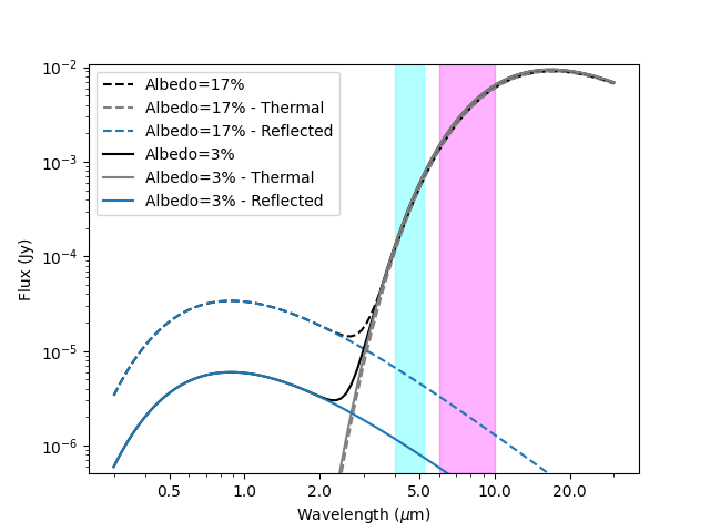
This is a plot of the total flux in Jy vs wavelength for 2 objects with different geometric albedos. This plot appears in several papers.

Color bands correspond to NEO Surveyor IR observation bands NC1 and NC2 respectively.

import numpy as np
import matplotlib.pyplot as plt
import kete


def flux_per_wavelength(
    phase=np.radians(90),
    solar_elong=np.radians(83),
    v_albedo=0.17,
    diameter=0.140,
    wavelength=np.logspace(np.log10(300), np.log10(30000), 100),
):
    """
    Calculate the flux as a function of wavelength.

    Parameters
    ----------
    phase:
        The phase angle of the object.
    solar_elongation:
        The angle the object is away from the sun from the point of view of the Earth.
    albedo:
        The geometric albedo of the object, assumed to be the same for all wavelengths.
    diameter:
        The diameter of the object in km.
    wavelength:
        A list of wavelengths in nm.

    Returns:
    wavelengths:
        Returns the input wavelengths back.
    flux:
        The total NEATM + reflected flux from the object.
    """

    # Calculate the geometry, the observer is placed 1 AU from the sun.
    sun2sc = kete.Vector([1.0, 0, 0])

    alpha = np.pi - phase - solar_elong
    peri_dist = sun2sc.r / np.sin(phase) * np.sin(solar_elong)

    sun2obj = kete.Vector([np.cos(alpha) * peri_dist, np.sin(alpha) * peri_dist, 0])

    fluxes = []
    for wave in wavelength:
        flux = kete.flux.neatm_flux(
            sun2obj,
            sun2sc,
            v_albedo=v_albedo,
            g_param=0.15,
            beaming=1.5,
            diameter=diameter,
            wavelength=wave,
            emissivity=0.9,
        )
        refl_flux = kete.flux.hg_apparent_flux(
            sun2obj,
            sun2sc,
            g_param=0.15,
            diameter=diameter,
            wavelength=wave,
            v_albedo=v_albedo,
        )
        fluxes.append((flux, refl_flux))

    return wavelength, np.array(fluxes)


# The values selected here were chosen to closely match the previously circulated plot.
y_min = 1000
y_max = 0
for ls, albedo in zip(["--", "-"], [0.17, 0.03]):
    wavelength, fluxes = flux_per_wavelength(v_albedo=albedo)
    total_flux = np.sum(fluxes, axis=1)
    plt.plot(
        wavelength / 1000,
        total_flux,
        label=f"Albedo={albedo * 100:0.0f}%",
        ls=ls,
        color="black",
    )
    y_min = min([y_min, np.min(total_flux)])
    y_max = max([y_max, np.max(total_flux)])
    plt.plot(
        wavelength / 1000,
        fluxes[:, 0],
        label=f"Albedo={albedo * 100:0.0f}% - Thermal",
        ls=ls,
        color="grey",
    )
    plt.plot(
        wavelength / 1000,
        fluxes[:, 1],
        label=f"Albedo={albedo * 100:0.0f}% - Reflected",
        ls=ls,
        color="C0",
    )
plt.ylabel("Flux (Jy)")
plt.xlabel(r"Wavelength ($\mu$m)")
plt.legend()
plt.yscale("log")
plt.xscale("log")
plt.xticks([0.5, 1.0, 2.0, 5.0, 10.0, 20.0], [0.5, 1.0, 2.0, 5.0, 10.0, 20.0])
plt.ylim(y_min * 0.85, y_max * 1.15)
plt.fill_between(
    [4, 5.2], [1], color="cyan", alpha=0.3, transform=plt.gca().get_xaxis_transform()
)
plt.fill_between(
    [6, 10], [1], color="magenta", alpha=0.3, transform=plt.gca().get_xaxis_transform()
)
plt.show()