Plotting Jupiter Trojans

import kete
import numpy as np
import matplotlib.pyplot as plt

# Load orbit data and select just the jupiter trojans
orbs = kete.mpc.fetch_known_orbit_data()
subset = orbs[kete.population.jup_trojan(orbs.peri_dist, orbs.ecc)]

# Construct the states and propagate them to a common epoch
states = kete.mpc.table_to_states(subset)
states = kete.propagate_n_body(states, states[0].jd)

# Where is jupiter?
jupiter = kete.spice.get_state("Jupiter", states[0].jd)
# found it!

# Compute the positions, and relative longitudinal distance from jupiter
positions = np.transpose([[s.pos.x, s.pos.y] for s in states])

longitudes = np.array([(s.pos.lon - jupiter.pos.lon + 180) % 360 - 180 for s in states])
leading = longitudes > 0
trailing = longitudes < 0

# Plot the results

Histogram of Trojan counts

plt.figure(figsize=(6, 4), dpi=150)
bins = np.linspace(-180, 180, 120)
plt.hist(longitudes[leading], bins=bins, histtype="step", color="C0")
plt.hist(longitudes[trailing], bins=bins, histtype="step", color="C2")
plt.title("Jupiter Trojans")
plt.xlabel("Ecliptic Lon away from Jupiter (Deg)")
plt.ylabel("Counts")

print(
    "Fraction of trojans which are in the leading camp: "
    f"{sum(leading) / len(longitudes):0.2%}"
)
plt.show()

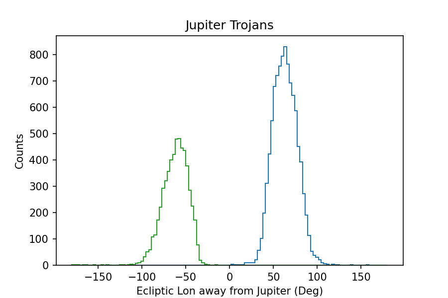
Fraction of trojans which are in the leading camp: 63.92%

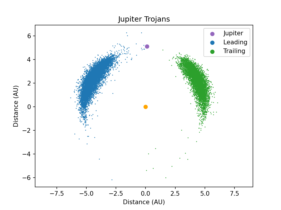
Top down view of the solar system

plt.figure(dpi=150)
plt.scatter(*positions[:, leading], s=0.2, c="C0")
plt.scatter(*positions[:, trailing], s=0.2, c="C2")
plt.scatter(jupiter.pos.x, jupiter.pos.y, c="C4", label="Jupiter")
plt.scatter(0, 0, c="Orange")
plt.scatter([], [], c="C0", label="Leading")
plt.scatter([], [], c="C2", label="Trailing")
plt.gca().axis("equal")
plt.legend()
plt.xlabel("Distance (AU)")
plt.ylabel("Distance (AU)")
plt.title("Jupiter Trojans")
plt.show()