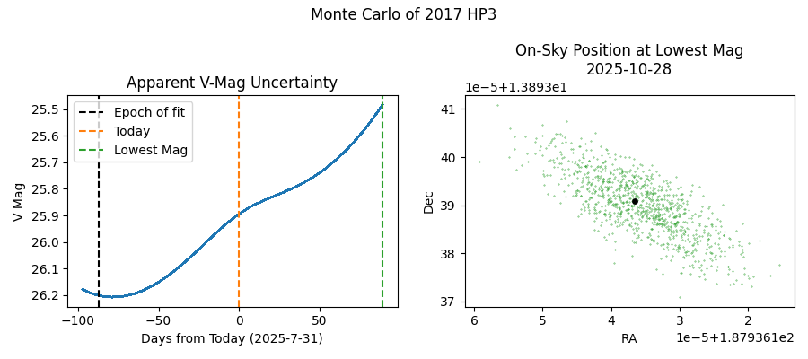
Plot On-Sky Uncertainty

This is inspired by the JPL Scout service, running Monte Carlo of the covariance matrix of the orbit fit.

import matplotlib.pyplot as plt
import numpy as np
import kete

# Inputs:
# -------

obj_name = "2017 HP3"

days_into_future = 90
time_step = 3

n_samples = 1000


# Calculating Samples
# -------------------
obj = kete.HorizonsProperties.fetch(obj_name)
g = obj.g_phase if obj.g_phase else 0.15

# Sample time
cur_jd = kete.Time.now().jd
jd_e = cur_jd + days_into_future
jd_s = obj.epoch - 10
jds = np.arange(jd_s, jd_e, time_step)

# Sample the covariance matrix
cov = np.array(obj.covariance.cov_matrix)
samples = kete.covariance.generate_sample_from_cov(n_samples, cov)
labels, values = zip(*obj.covariance.params)
values = np.array(values)

# Construct new states from the covariance samples.
# Keep the current best estimate as the first state.
states = [obj.state]
for sample in samples:
    sample = sample + values
    params = dict(zip(labels, sample))
    states.append(kete.CometElements(obj.desig, obj.covariance.epoch, **params).state)

# Propagate the position of all states to all time steps, recording the V mags
mags = []
for jd in jds:
    states = kete.propagate_n_body(states, jd)
    earth = kete.spice.get_state("earth", jd)
    m = [
        kete.flux.hg_apparent_mag(
            sun2obj=x.pos, sun2obs=earth.pos, h_mag=obj.h_mag, g_param=g
        )
        for x in states
    ]
    mags.append(m)

# Find the step where the median magnitude was the brightest
brightest_idx = np.argmin(np.median(mags, axis=1))
brightest_jd = jds[brightest_idx]

# position at lowest mag
states = kete.propagate_n_body(states, brightest_jd)
earth = kete.spice.get_state("earth", brightest_jd)
vecs = [(s.pos - earth.pos).as_equatorial for s in states]
ras = np.array([v.ra for v in vecs])
decs = np.array([v.dec for v in vecs])


# Plotting Results
# ----------------
plt.figure(figsize=(9, 4))

plt.suptitle(f"Monte Carlo of {obj.desig}")

plt.subplot(1, 2, 1)
plt.title("Apparent V-Mag Uncertainty")

plt.plot(jds - cur_jd, mags, c="C0", alpha=0.05)

plt.ylabel("V Mag")
ymd_today = "-".join(f"{x:0.0f}" for x in kete.Time(cur_jd).ymd)
plt.xlabel(f"Days from Today ({ymd_today})")

plt.axvline(obj.epoch - cur_jd, ls="--", label="Epoch of fit", c="k")
plt.axvline(0, ls="--", label="Today", c="C1")
plt.axvline(brightest_jd - cur_jd, ls="--", label="Lowest Mag", c="C2")

plt.legend()
plt.gca().invert_yaxis()

# Little bit of trickery to make plotting prettier.
#
# This sorts all ra, dec pairs by the dec value, and unwraps
# periodic valus of ra. What this means is that if ra has
# a collection of points split across the 0-360 boundary it will
# plot around either 0 or 360 as a single blob and extend either to
# negative angles or above 360.
idx_sort = np.argsort(ras)
decs = decs[idx_sort]
ras = np.unwrap(ras[idx_sort], period=360)
ymd = "-".join(f"{x:0.0f}" for x in kete.Time(brightest_jd).ymd)

plt.subplot(1, 2, 2)
plt.title(f"On-Sky Position at Lowest Mag\n{ymd}")
plt.scatter(ras, decs, s=0.1, c="C2")

plt.scatter(vecs[0].ra, vecs[0].dec, s=15, c="k")
plt.xlabel("RA")
plt.ylabel("Dec")
plt.gca().invert_xaxis()
plt.tight_layout()
plt.show()